Plant Disease Detection using the PlantDoc Dataset and PyTorch Faster RCNN

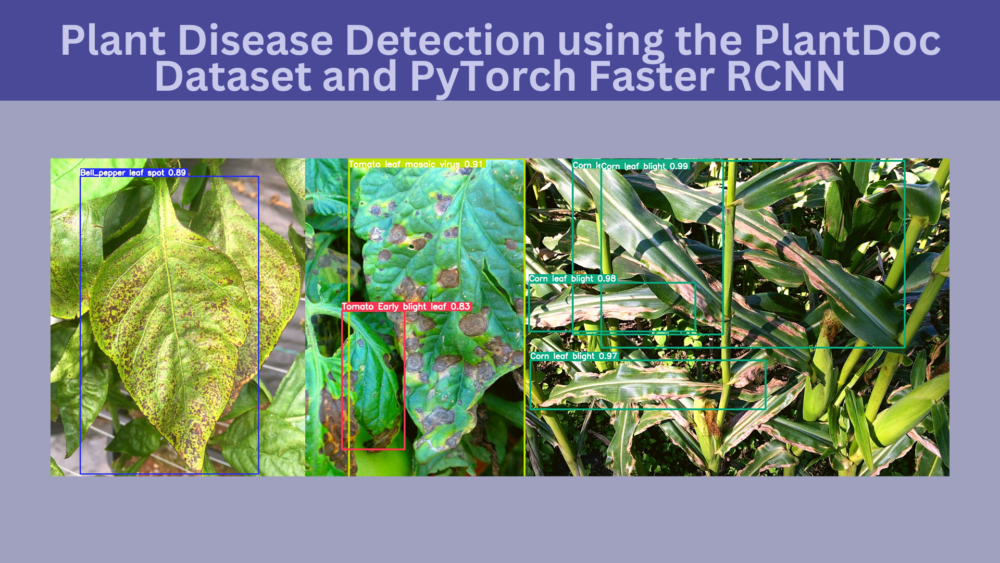
Recognizing plant disease can lead to faster treatment which can result in better yields. In the last two blog posts, we have already seen how deep learning and computer vision can help in recognizing different plant diseases effectively. In this post, we will march on a much more challenging problem. That is plant disease detection. We will use the PlantDoc dataset for plant disease detection with the PyTorch Faster RCNN ResNet50 FPN V2 model.

Detection of plant disease can prove to be much more effective compared to disease recognition (classification). Object detection can point out which parts or leaves of the plant are affected and with which disease. This although a very effective solution, as we will later on see, is much more challenging as well.

For now, let’s check all the points that we will cover in this post:

• We will start with a discussion of the PlantDoc dataset for Plant Disease Detection.
• Then we will go over the reasons to choose the PyTorch Faster RCNN model for this project. Also, we will get familiar with the codebase that we will use to train the model.
• After that, we will check the directory structure of the project.
• Then we will move on to training the Faster RCNN model on the PlantDoc dataset for plant disease detection.
• Next, we will analyze the results and run inference on images from the internet.

The PlantDoc Detection Dataset

The PlantDoc dataset has two versions, one for disease recognition and one for disease detection. In this post, we will use the PlantDoc dataset for disease detection. You can find the official GitHub repository for the same here.

It also has an accompanying paper called PlantDoc: A Dataset for Visual Plant Disease Detection. You can give the paper a read to know the benchmarks and results of the authors.

But instead of using the dataset from the GitHub repository, we will be using a resized version of it. You will have access to the dataset files along with the source code in the download section of the post.

The PlantDoc dataset has 30 object classes. But all the classes do not contain the same number of images. This is what makes this dataset so much harder to learn for object detection models.

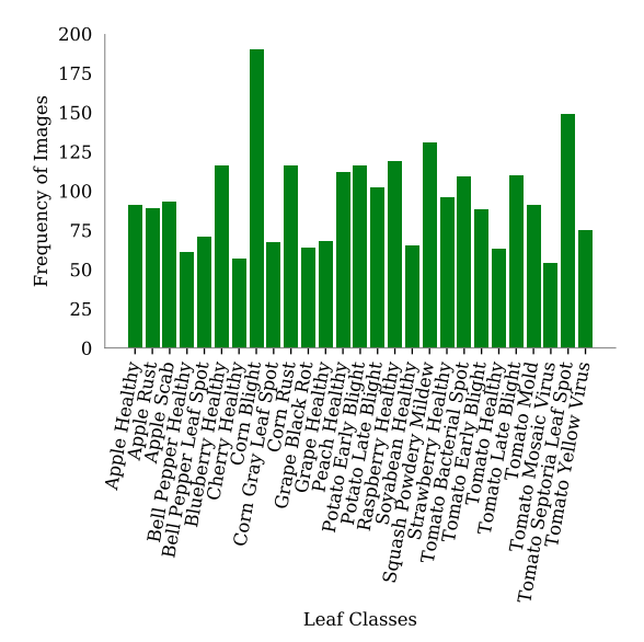
As you may observe in the above graph, some classes have as high as 180 images, while some have as low as 50 images. Plant disease detection already being a difficult problem, and an unbalanced dataset makes it even more challenging.

Still, we will try our best to train a Faster RCNN ResNet50 FPN V2 model using PyTorch and get good results.

Following are some of the images from the training with their annotations.

As you can see, the leaves with diseases have the disease name attached to the leaf name. Leaves without any disease have been annotated with just the leaf name.

The dataset has already been divided into training and test set. The training set contains 2328 images and the test set contains 237 images.

Knowledge Augmentation

Before moving further, if you are interested to know about plant disease recognition using different models, then these two articles are just for you.

• PlantVillage Dataset Disease Recognition using PyTorch
• PlantDoc Dataset for Plant Disease Recognition using PyTorch

The above two articles will reinforce how different models perform on the PlantVillage and PlantDoc recognition datasets. Also, we experiment and train various models like:

• EfficientNets
• ResNets
• MobileNets

Why the PyTorch Faster RCNN ResNet50 FPN Model?

Plant disease detection is a challenging problem. The disease can affect both, the leaves and the fruits of the plants. Not to mention the complex and varied backgrounds which the image may contain. And of course, the lack of diverse and big datasets for plant disease detection.

Due to these reasons, we need a pretty good object detection model. The Faster RCNN models from PyTorch are good at handling complex datasets even with small objects. Therefore, we choose the Faster RCNN ResNet50 FPN V2 model for this purpose.

We will not be writing all the code from scratch. Instead, we will use this Faster RCNN Training Pipeline repository. It has been specifically developed to make Faster RCNN object detection training easier with different backbones.

Along with supporting various models, it also has local and Weight&Biases support so that we never lose experimental details.

We will clone this repository and make the necessary modifications before training the PlantDoc dataset for plant disease detection. Any other details related to the code and training of the model, we will discuss them as we move along.

Setting the Code Repository

For now, you can go ahead and clone the repository in the directory of your choice.

git clone https://github.com/sovit-123/fasterrcnn-pytorch-training-pipeline.git

If you are using the Linux OS and have CUDA and cuDNN already installed, you can right away install the requirements in the environment of your choice. Just execute the following command inside the fasterrcnn-pytorch-training-pipeline directory.

The code requires PyTorch >= 1.12.0 to run properly. This is because we will use the latest API to load the IMAGENET1KV1 and IMAGENET1KV2 weights.

pip install -r requirements.txt

If you are using the Windows OS, do check out this section in the README file for the complete setup guidelines.

Directory Structure

Let’s take a look at the directory structure for this project.

.
├── fasterrcnn-pytorch-training-pipeline
│   ├── data
│   ├── data_configs
│   │   ├── aquarium.yaml
│   │   ...
│   │   ├── plantdoc.yaml
│   │   ...
│   │   └── voc.yaml
│   ├── models [26 entries exceeds filelimit, not opening dir]
│   ├── notebook_examples
│   │   ...
│   │   └── visualizations_plantdoc.ipynb
│   ├── outputs
│   │   ├── inference
│   │   │   ├── res_1
│   │   │   ...
│   │   └── training
│   │       └── fasterrcnn_resnet50_fpn_v2_trainaug_30e
│   ├── torch_utils
│   │   ├── coco_eval.py
│   │   ...
│   │   ├── __init__.py
│   │   └── utils.py
│   ├── utils
│   │   ...
│   │   └── validate.py
│   ├── datasets.py
│   ├── eval.py
│   ├── inference.py
│   ├── inference_video.py
│   ├── __init__.py
│   ├── requirements.txt
│   └── train.py
└── input
    ├── inference_data
    │    |── images
    │       ├── apple_rust.png
    │       ...
    │       └── tomato_early_blight.jpg
    └── plantdoc_resized_416_416
        ├── test
        │   ├── images
        │   └── labels
        └── train
            ├── images
            └── labels

• The fasterrcnn-pytorch-training-pipeline directory is the repository that we cloned above. It contains several directories and files. But the most important ones are the data_configs directory, train.py, inference.py, and inference_video.py files.
• The data_configs directory holds the YAML file for specific datasets. These YAML files hold the training/validation data paths, the class names, and the number of classes. For this particular project, we are interested in the plantdoc.yaml file.
• For training, we will use the train.py file. The inference.py and inference_video.py files are for running inference on images and videos respectively.
• Coming to the input directory in the project folder. The inference_data subdirectory contains a few images for inference. The plantdoc_resized_416_416 subdirectory contains the training and test data. The images and XML label files are in their respective folders.

The training and inference data will be available to download in this blog post. In case you wish to run the code locally, you need to clone the repository and install the requirements as discussed in the previous section.

Plant Disease Detection using the PlantDoc Dataset with PyTorch and Faster RCNN

Without any delay, let’s jump into the practical side of this post.

Download Code

Preparing the Dataset YAML File

For training a plant disease detection model on the PlantDoc dataset, first, we have to set up a dataset YAML file. This file will reside in the fasterrcnn-pytorch-training-pipeline/data_configs directory.

For this project, we are calling it plantdoc.yaml file. Here is the entire content of the file.

# Images and labels direcotry should be relative to train.py
TRAIN_DIR_IMAGES: '../input/plantdoc_resized_416_416/train/images'
TRAIN_DIR_LABELS: '../input/plantdoc_resized_416_416/train/labels'
VALID_DIR_IMAGES: '../input/plantdoc_resized_416_416/test/images'
VALID_DIR_LABELS: '../input/plantdoc_resized_416_416/test/labels'

# Class names.
CLASSES: [
    '__background__',
    'Apple Scab Leaf', 'Apple leaf', 'Apple rust leaf', 
    'Bell_pepper leaf spot', 'Bell_pepper leaf', 'Blueberry leaf',
    'Cherry leaf', 'Corn Gray leaf spot', 'Corn leaf blight', 
    'Corn rust leaf', 'Peach leaf', 'Potato leaf early blight',
    'Potato leaf late blight', 'Potato leaf', 'Raspberry leaf',
    'Soyabean leaf', 'Soybean leaf', 'Squash Powdery mildew leaf',
    'Strawberry leaf', 'Tomato Early blight leaf', 
    'Tomato Septoria leaf spot', 'Tomato leaf bacterial spot', 
    'Tomato leaf late blight', 'Tomato leaf mosaic virus', 
    'Tomato leaf yellow virus', 'Tomato leaf', 'Tomato mold leaf', 
    'Tomato two spotted spider mites leaf', 'grape leaf black rot', 'grape leaf'
    ]

# Number of classes (object classes + 1 for background class in Faster RCNN).
NC: 31

# Whether to save the predictions of the validation set while training.
SAVE_VALID_PREDICTION_IMAGES: True

We provide the training and validation paths for the images and the labels. These paths are relative to the fasterrcnn-pytorch-training-pipeline directory from where we will execute the train.py script. We also list out the class names and the total number of classes in this YAML file.

Frankly, this is the only file that we need to prepare to train a model using the code of this repository.

In that case, why don’t we jump directly into training?

Training the Faster RCNN ResNet50 FPN V2 Model on the PlantDoc Dataset

To start the training, we need to execute the train.py file within the cloned repository. The following code block contains the entire training command.

python train.py --model fasterrcnn_resnet50_fpn_v2 --epochs 30 --data data_configs/plantdoc.yaml --no-mosaic --use-train-aug --name fasterrcnn_resnet50_fpn_v2_trainaug_30e

As you may see, the command contains quite a lot of arguments. The following are the explanations for each of them.

• --model: This is the model that we want to use to train on the dataset. We choose the Faster RCNN ResNet50 FPN V2 for this purpose. As this is a PyTorch pretrained model, the weights will be automatically downloaded or used from the cache.
• --epochs: The number of epochs that we want to train for.
• --data: This flag accepts the path to the dataset YAML file. Here, we provide the path to the plantdoc.yaml file that we prepared in the previous section.
• --no-mosaic: The code in this repository supports mosaic augmentation and also applies it by default. But we are turning it off.
• --use-train-aug: Although we do not apply the mosaic augmentation, we apply several other augmentations using albumentations for object detection. You may check out transforms.py file to get into the details.
• --name: Giving an elaborate name to the project will help us differentiate it easily when carrying out multiple experiments. The outputs of this training will be saved in a folder with this name inside the outputs/training directory.

The above are all the command line arguments that we use. In case, you wish to know about all the flags, please check them out in the train.py file.

Training Results After Training on the PlantDoc Dataset for Plant Disease Detection

The following is the truncated output from the terminal.

Not using distributed mode
device cuda
Creating data loaders
Number of training samples: 2328
Number of validation samples: 239
.
.
.
 Average Precision  (AP) @[ IoU=0.50:0.95 | area=   all | maxDets=100 ] = 0.383
 Average Precision  (AP) @[ IoU=0.50      | area=   all | maxDets=100 ] = 0.509
 Average Precision  (AP) @[ IoU=0.75      | area=   all | maxDets=100 ] = 0.444
 Average Precision  (AP) @[ IoU=0.50:0.95 | area= small | maxDets=100 ] = -1.000
 Average Precision  (AP) @[ IoU=0.50:0.95 | area=medium | maxDets=100 ] = 0.095
 Average Precision  (AP) @[ IoU=0.50:0.95 | area= large | maxDets=100 ] = 0.389
 Average Recall     (AR) @[ IoU=0.50:0.95 | area=   all | maxDets=  1 ] = 0.457
 Average Recall     (AR) @[ IoU=0.50:0.95 | area=   all | maxDets= 10 ] = 0.619
 Average Recall     (AR) @[ IoU=0.50:0.95 | area=   all | maxDets=100 ] = 0.622
 Average Recall     (AR) @[ IoU=0.50:0.95 | area= small | maxDets=100 ] = -1.000
 Average Recall     (AR) @[ IoU=0.50:0.95 | area=medium | maxDets=100 ] = 0.223
 Average Recall     (AR) @[ IoU=0.50:0.95 | area= large | maxDets=100 ] = 0.634
SAVING PLOTS COMPLETE...
SAVING PLOTS COMPLETE...
SAVING PLOTS COMPLETE...
SAVING PLOTS COMPLETE...
SAVING PLOTS COMPLETE...
SAVING PLOTS COMPLETE...

As usual, we use the Mean Average Precision (mAP) as the object detection metric here. After the final epoch, the mAP is 38.3. But this is not the mAP for the best epoch. The model achieves the best mAP after epoch 24 where the mAP was 40.3.

IoU metric: bbox
 Average Precision  (AP) @[ IoU=0.50:0.95 | area=   all | maxDets=100 ] = 0.403
 Average Precision  (AP) @[ IoU=0.50      | area=   all | maxDets=100 ] = 0.533
 Average Precision  (AP) @[ IoU=0.75      | area=   all | maxDets=100 ] = 0.476
 Average Precision  (AP) @[ IoU=0.50:0.95 | area= small | maxDets=100 ] = -1.000
 Average Precision  (AP) @[ IoU=0.50:0.95 | area=medium | maxDets=100 ] = 0.076
 Average Precision  (AP) @[ IoU=0.50:0.95 | area= large | maxDets=100 ] = 0.412
 Average Recall     (AR) @[ IoU=0.50:0.95 | area=   all | maxDets=  1 ] = 0.480
 Average Recall     (AR) @[ IoU=0.50:0.95 | area=   all | maxDets= 10 ] = 0.636
 Average Recall     (AR) @[ IoU=0.50:0.95 | area=   all | maxDets=100 ] = 0.638
 Average Recall     (AR) @[ IoU=0.50:0.95 | area= small | maxDets=100 ] = -1.000
 Average Recall     (AR) @[ IoU=0.50:0.95 | area=medium | maxDets=100 ] = 0.225
 Average Recall     (AR) @[ IoU=0.50:0.95 | area= large | maxDets=100 ] = 0.646

Later, when running inference on images for plant disease detection, we will use this best model only.

The following image shows the mAP graph over the entire training.

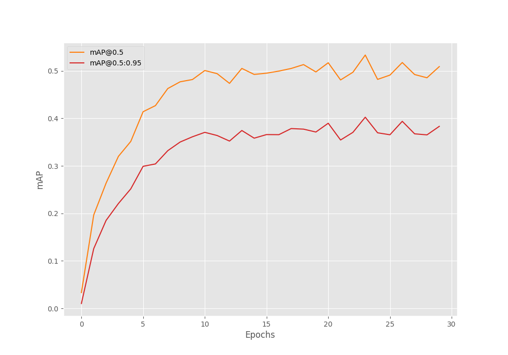
It is difficult to say whether we could have trained longer without overfitting. We can surely try, and because the best model is always getting saved to disk, we do not need to worry about getting the overfitted model. Also, we have to option to stop the training now, and again resume it with mosaic augmentations which may improve the results.

Running Evaluation on the Test Set

We can also run evaluation using the best model. As we do not have a separate validation set, the evaluation script will use the same test data. So, we should get the same mAP that we got after epoch 24, which is 40.3.

We can use the eval.py script to run the evaluation.

python eval.py --model fasterrcnn_resnet50_fpn_v2 --weights outputs/training/fasterrcnn_resnet50_fpn_v2_trainaug_30e/best_model.pth --data data_configs/plantdoc.yaml 

{'map': tensor(0.4030),
 'map_50': tensor(0.5338),
 'map_75': tensor(0.4764),
 'map_large': tensor(0.4120),
 'map_medium': tensor(0.0763),
 'map_per_class': tensor(-1.),
 'map_small': tensor(-1.),
 'mar_1': tensor(0.4805),
 'mar_10': tensor(0.6366),
 'mar_100': tensor(0.6386),
 'mar_100_per_class': tensor(-1.),
 'mar_large': tensor(0.6467),
 'mar_medium': tensor(0.2248),
 'mar_small': tensor(-1.)}

The evaluation script uses Torchmetrics to compute the mAP. And as you can see, we get 40.3 mAP here again.

Running Inference on Images for Plant Disease Detection

Let’s start with running inference on images. Right now, we have a model which has been trained on the PlantDoc plant disease detection dataset. We will use the best model that has been saved for running inference on a few images from the internet.

We can use the inference.py script for this. You can run the following command inside the fasterrcnn-pytorch-training-pipeline directory.

python inference.py --weights outputs/training/fasterrcnn_resnet50_fpn_v2_trainaug_30e/best_model.pth --input ../input/inference_data/images/ --threshold 0.8 --imgsz 640

The following are the explanations of the command line flags.

• --weights: This flag accepts the path to the model weights that we want to use for inference.
• --input: This flag accepts the path to either a directory containing images or a single image. Here, we are providing the path to a directory containing images.
• --threshold: This is the visualization threshold that we set. Any detections having a confidence score below 0.8 will be dropped.
• --imgsz: The size we want the images to be resized to. As the model has been trained on 640×640 images, we are resizing it to the same size during inference to get the best results.

We can find the outputs in a folder inside the outputs/inference directory.

Inference Results

Here, are the results that we get. The blue text on the top of each image shows the ground truth disease. And the annotations are from the detections made by the model.

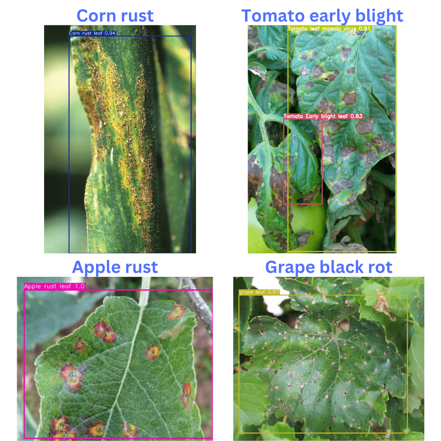
The model is performing pretty well here, given that these images are completely new for the model. It is detecting apple rust, and corn rust correctly. However, it is unable to detect the grape black rot disease and is misclassifying it as a healthy grape leaf.

For the tomato early blight disease also, it is only partially correct. It is detecting only one leaf with tomato early blight and missing out on a few others. Also, although a tomato leaf disease, the model is misclassifying another leaf as tomato leaf mosaic virus.

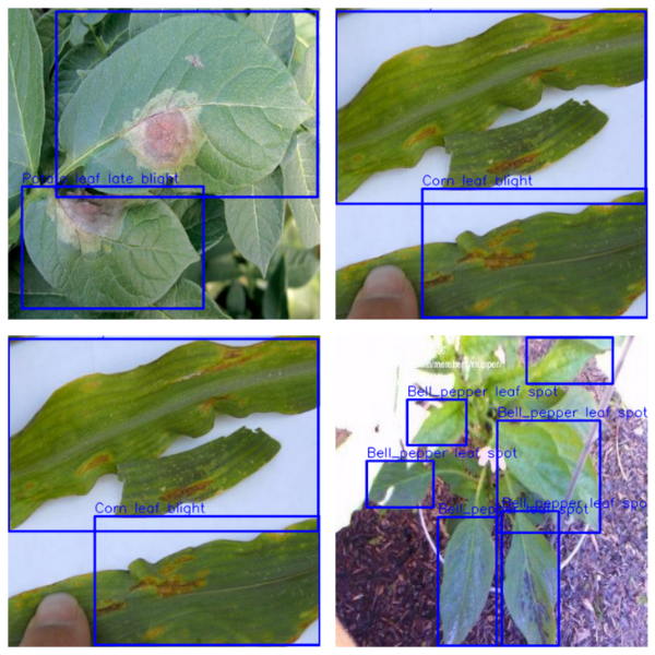
Here are a few more results after running inference on other images.

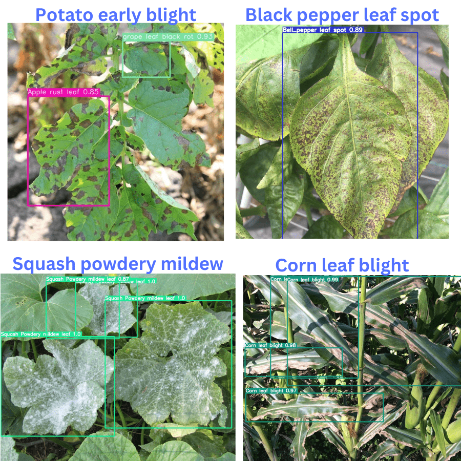
Interestingly, out of these 4 images, it is correctly detecting the diseases in 3 of them. The potato early blight is the only disease that it is wrongly detecting.

Takeaways

Carrying out the training and inference experiments using the PlantDoc dataset has given us some ideas about how challenging this can be. Even big deep learning models like Faster RCNN cannot be 100% accurate all the time.

Deep learning can obviously help in plant disease recognition and detection, but we will need much larger, better datasets along with well-trained models.

With proper datasets, we can target specific diseases, like apple scab detection and apple scab recognition.

Active research, experiments, and applying the new concepts of deep learning to solve this is the only way to go from here. In case you build anything interesting by taking this project forward, do let others know in the comment section.

Summary and Conclusion

In this blog post, we took on the challenge of training an object detection model on the PlantDoc dataset. After training the Faster RCNN ResNet50 FPN V2 on the dataset, we ran inference experiments on real-world images of leaves affected by various diseases. This gave us an idea of where the model was succeeding and where it was failing. Hopefully, this post was worthwhile for you.

In case you have any doubts, thoughts, or suggestions, please leave them in the comment section. I will surely address them.

You can contact me using the Contact section. You can also find me on LinkedIn, and Twitter.