PyTorch Pretrained EfficientNet Model Image Classification

Since we started to use deep learning for computer vision tasks, many new models have come up that exceed the performance of the previous models. Image classification and recognition is a major challenge in deep learning. And it has seen quite a few advancements in recent years. Thanks to the ImageNet dataset and the ILSVRC, both of which are great driving forces in the field. With that, in recent years, the new EfficientNet models have come up. These beat many previous state-of-the-art models in image classification. And with the recent release of PyTorch 1.10 (at the time of writing this), we now have access to all the EfficientNet models. In this tutorial, we will be carrying out image classification using PyTorch pretrained EfficientNet model.

Not only that, but we will also compare the forward pass time of EfficientNetB0 with the very famous ResNet50.

Let’s take look at all the points that we will cover in this post.

• We will start with a brief introduction to the EfficientNet models.
• Then we will see what all EfficientNet pretrained models PyTorch provides.
• In the coding section, we will load the EfficientNetB0 model to carry out image classification.
• Then we will compare the CPU and GPU timings for forward pass of EfficientNetB0 with that of ResNet50.

Let’s get into the details of the post now.

The EfficientNet Models

The EfficientNet models were introduced by Mingxing Tan and Quoc V. Le in the paper EfficientNet: Rethinking Model Scaling for Convolutional Neural Networks in 2019. Although a few years old by now, still, they are some of the best image classification models out there.

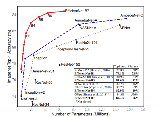
The EfficientNet models were able to beat most of the state-of-the-art deep learning models for image classification and recognition at the time. And from figure 2, we can also see that they were a family of 8 models starting from EfficientNetB0 to EfficientNetB7.

We can see that the number of parameters of the EfficientNet models was substantially less than other models. Still, they were ahead of the other models in terms of accuracy.

This was because of how the models were built. Without going into too many details, the authors used Neural Architecture Search (NAS) and compound scaling to discover the EfficientNet family of networks. Even the biggest of the EfficientNet model, that is, EfficientNetB7 achieves state-of-the-art 84.3% top-1 accuracy on ImageNet while being 8.4x smaller and 6.1x faster on inference compared to GPipe with 556 million parameters.

We will not go into any more details of the EfficientNet paper here. That requires its own dedicated post. Let’s move on to the pre-trained models provided by PyTorch.

PyTorch Pretrained EfficientNet Models

Starting with PyTorch version 1.10, we now have access to the pretrained EfficientNet models. We can access the models using the torchvision library of PyTorch. In fact, PyTorch provides all the models, starting from EfficientNetB0 to EfficientNetB7 trained on the ImageNet dataset.

This means that either we can directly load and use these models for image classification tasks if our requirement matches that of the pretrained models. Or we can also use these for transfer learning and fine-tuning on our own dataset.

In this post, we will carry out image classification using EfficientNetB0 and also compare the CPU and GPU forward pass time with that of ResNet50. Why ResNet50? We will answer that when carrying out that part.

For now, if you do not have PyTorch on your system, or have an older version, then please consider installing the latest version of PyTorch before moving further.

The Directory Structure

The following block shows the directory structure for the files/folders in this post.

├── input
│   ├── image_1.jpg
│   ├── image_2.jpg
│   └── image_3.jpg
├── outputs
│   ├── image_1_cpu.jpg
│   ├── image_1_cuda.jpg
│   ...
│   ├── time_vs_iterations_cpu.png
│   └── time_vs_iterations_cuda.png
├── compare.py
├── efficient_classification.py
├── imagenet_classes.txt
└── utils.py

• The input folder contains the three images that we will use for classification using the EfficientNetB0 model. These are images of a car, a dog, and a shark.
• The output folder will hold all the image classification outputs after running the code. It will also store the forward pass time comparison graphs for EfficientNetB0 vs ResNet50.
• We have three Python files and an imagenet_classes.txt file. This text file contains the 1000 ImageNet class names.

Downloading the zip file provided with this post will give you access to everything that we are using in this post. You just need to extract the file and you are all set up.

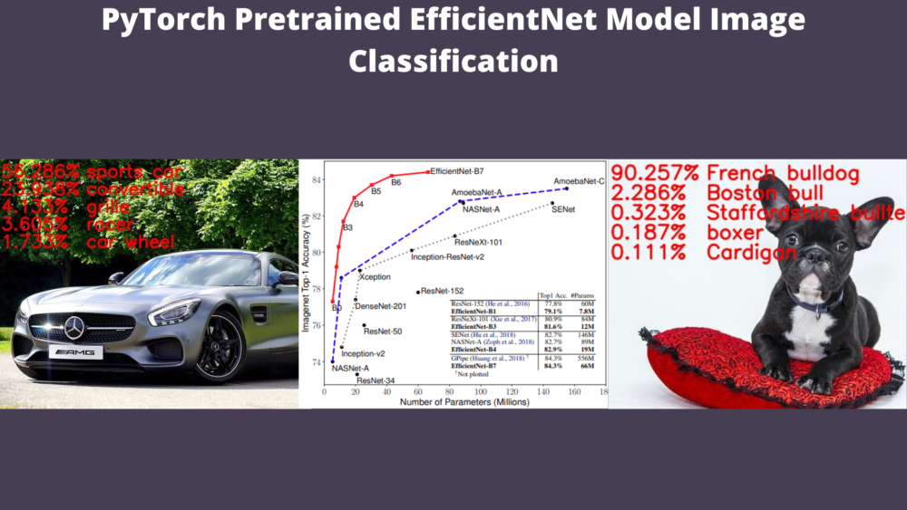
PyTorch Pretrained EfficientNet Model Image Classification

From here onward, we will start with the coding section of the tutorial. We will start with the image classification part using PyTorch pretrained EfficientNet model and then move on to comparing forward pass time between EfficientNetB0 and ResNet50.

Writing the Helper Functions

We will start with writing a few helper functions that we can reuse and also help us keep other parts of the code clean.

The code here will go into the utils.py file.

The first code block contains the import statements that we need.

import torchvision.models as models
import torch
import time
import matplotlib.pyplot as plt

from torchvision import transforms

plt.style.use('ggplot')

We need matplotlib to plot the time vs iteration graphs for the forward pass time of both EfficientNetB0 and ResNet50 models.

Next, we have two functions to load pretrained models from torchvision. One for EfficientNetB0 and another for ResNet50.

def load_efficientnet_model():
    """
    Load the pre-trained EfficientNetB0 model.
    """
    model = models.efficientnet_b0(pretrained=True)
    model.eval()
    return model

def load_resnet50_model():
    """
    Load the pre-trained ResNet50 model.
    """
    model = models.resnet50(pretrained=True)
    model.eval()
    return model

We are loading the pretrained ImageNet weights in both cases. Note that we need the ResNet50 model only for the comparison part. For standalone image classification, we will just use the EfficientNetB0 model.

The next function preprocesses the image before being fed into the neural network model. We also have another function to read the ImageNet classes from imagenet_classes.txt file.

def preprocess():
    """
    Define the transform for the input image/frames.
    Resize, crop, convert to tensor, and apply ImageNet normalization stats.
    """
    transform =  transforms.Compose([
        transforms.ToPILImage(),
        transforms.Resize(256),
        transforms.CenterCrop(224),
        transforms.ToTensor(),
        transforms.Normalize(mean=[0.485, 0.456, 0.406], 
                             std=[0.229, 0.224, 0.225]),])
    return transform

def read_classes():
    """
    Load the ImageNet class names.
    """
    with open("imagenet_classes.txt", "r") as f:
        categories = [s.strip() for s in f.readlines()]
    return categories

We are cropping the image, resizing it to 224×224, converting it to tensor, and applying the ImageNet normalization.

The final two functions are to carry out forward pass through the model multiple times and to plot the time vs iterations graph.

def run_through_model(model, input_batch, n_runs):
    """
    Forward passes the image tensor batch through the model 
    `n_runs` number if times. Prints the average milliseconds taken
    and returns a list containing all the forward pass times.
    """
    total_time = 0
    time_list = []
    for i in range(n_runs):
        print(f"Run: {i+1}", end='\r')
        with torch.no_grad():
            start_time = time.time()
            output = model(input_batch)
            end_time = time.time()
            time_list.append((end_time-start_time)*1000)
            total_time += (end_time - start_time)*1000

    print(f"{total_time/n_runs:.3f} milliseconds\n")
    return time_list

def plot_time_vs_iter(model_names, time_lists, device):
    """
    Plots the iteration vs time graph for given model.

    :param model_name: List of strings, name of both the models.
    :param time_list: List of lists, containing time take for each iteration
        for each model.
    :param device: Computation device.
    """
    colors = ['green', 'red']
    plt.figure(figsize=(10, 7))
    for i, name in enumerate(model_names):
        plt.plot(
            time_lists[i], color=colors[i], linestyle='-', 
            label=f"time taken (ms) {name}"
        )
    plt.xlabel('Iterations')
    plt.ylabel('Time Taken (ms)')
    plt.legend()
    plt.savefig(f"outputs/time_vs_iterations_{device}.png")
    plt.show()
    plt.close()

The run_through_model() function accepts the model, the input tensors, and n_runs, that is, the number of times to carry out forward pass through the model. We keep on appending the forward pass time to time_list so that we can plot graphs later. We also print the average time taken in milliseconds.

The plot_time_vs_iter() plots the time take for each of the iterations (each of n_runs) for both, the EfficientNetB0 as well as the ResNet50 model. Note that it accepts one device parameter as well that we use during saving the plot to disk. This is because we will run this experiment twice, once with CPU, and once with GPU.

The above are all the helper functions that we need for this post.

Image Classification using PyTorch Pretrained EfficientNet Model

Here, we will write the code to carry out image classification using the PyTorch pretrained EfficientNet model. This part is going to be easy as most of the work is already complete while writing the helper functions.

All the code here will go into the efficientnet_classification.py script.

Starting with the import statements and creating the argument parser.

import torch
import cv2
import argparse
import time

from utils import (
    load_efficientnet_model, preprocess, read_classes
)

# Construct the argumet parser to parse the command line arguments.
parser = argparse.ArgumentParser()
parser.add_argument('-i', '--input', default='input/image_1.jpg', 
                    help='path to the input image')
parser.add_argument('-d', '--device', default='cpu', 
                    help='computation device to use', 
                    choices=['cpu', 'cuda'])
args = vars(parser.parse_args())

We are importing the required functions from the utils module. For the argument parser, we have the following flags:

• --input: Path to the input image.
• --device: The computation device to use. Accepts either cpu or cuda.

Required Initializations and Set Up

Now, let’s set up all that we need before doing the forward pass.

# Set the computation device.
DEVICE = args['device']
# Initialize the model.
model = load_efficientnet_model()
# Load the ImageNet class names.
categories = read_classes()
# Initialize the image transforms.
transform = preprocess()

print(f"Computation device: {DEVICE}")

image = cv2.imread(args['input'])
rgb_image = cv2.cvtColor(image, cv2.COLOR_BGR2RGB)
# Apply transforms to the input image.
input_tensor = transform(image)
# Add the batch dimension.
input_batch = input_tensor.unsqueeze(0)

# Move the input tensor and model to the computation device.
input_batch = input_batch.to(DEVICE)
model.to(DEVICE)

In the above code block, we start with setting up the computation device. Then we load the model on line 21, read the image classes on line 23, and initialize the transforms.

Starting from line 29, we read the image, convert it to RGB color format, apply the transforms, and add the batch dimension. Then we load the input tensor to the computation device.

Forward Pass

Now, it’s time to forward pass the input through the model and check out the predictions.

with torch.no_grad():
    start_time = time.time()
    output = model(input_batch)
    end_time = time.time()

# Get the softmax probabilities.
probabilities = torch.nn.functional.softmax(output[0], dim=0)

# Check the top 5 categories that are predicted.
top5_prob, top5_catid = torch.topk(probabilities, 5)
for i in range(top5_prob.size(0)):
    cv2.putText(image, f"{top5_prob[i].item()*100:.3f}%", (15, (i+1)*30), 
                cv2.FONT_HERSHEY_SIMPLEX,
                1, (0, 0, 255), 2, cv2.LINE_AA)
    cv2.putText(image, f"{categories[top5_catid[i]]}", (160, (i+1)*30), 
                cv2.FONT_HERSHEY_SIMPLEX,
                1, (0, 0, 255), 2, cv2.LINE_AA)
    print(categories[top5_catid[i]], top5_prob[i].item())

cv2.imshow('Result', image)
cv2.waitKey(0)

# Define the outfile file name.
save_name = f"outputs/{args['input'].split('/')[-1].split('.')[0]}_{DEVICE}.jpg"
cv2.imwrite(save_name, image)
print(f"Forward pass time: {(end_time-start_time):.3f} seconds")

The forward pass happens on line 41. We also calculate the time taken for the forward pass. We calculate the Softmax probabilities of the outputs on line 45. On line 48, we extract the top 5 probabilities and their respective class names. After that, starting from line 49, we are annotating the image with the top 5 predicted class names and the probabilities. Finally, we show the result on the screen, save the resulting image to disk, and also show the forward pass time in seconds.

This is all we need for image classification using PyTorch pretrained EfficientNet model.

Execute efficientnet_classification.py File

All the experiments have been performed on a system with the following hardware configuration.

• Intel Core i7 10700K.
• 32 GB RAM.
• RTX 3080 GPU.

Now, it’s time to execute the efficientnet_classification.py while providing the images we have in the input folder and check out the predictions.

First, we will run all predictions on the CPU, then on the GPU.

Open the terminal/command line in the parent project directory. Let’s start with image_1.jpg.

python efficientnet_classification.py --input input/image_1.jpg --device cpu

The following is the output on the terminal.

Computation device: cpu
sports car 0.5628593564033508
convertible 0.23938272893428802
grille 0.04133297875523567
racer 0.03605145588517189
car wheel 0.017325162887573242
Forward pass time: 0.015 seconds

And the following is the resulting output image.

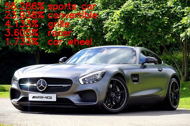
We can see that the EfficientNetB0 model predicted the image as sports car with 56% probability. This seems to be correct. And the forward pass time is 0.015 seconds which looks really good.

Let’s try out the other images.

python efficientnet_classification.py --input input/image_2.jpg --device cpu

The output on the terminal.

Computation device: cpu
French bulldog 0.9025659561157227
Boston bull 0.022857174277305603
Staffordshire bullterrier 0.003226602915674448
boxer 0.0018747287103906274
Cardigan 0.0011134210508316755
Forward pass time: 0.014 seconds

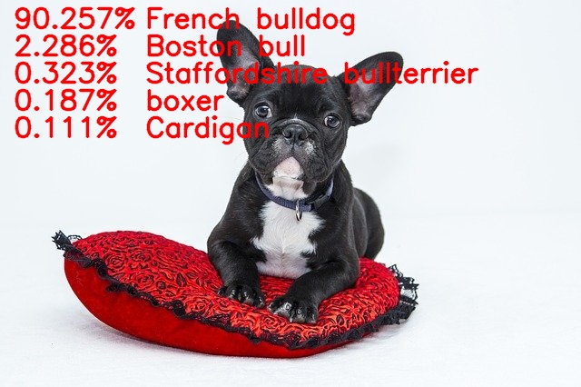
This time also the French bulldog prediction looks correct.

python efficientnet_classification.py --input input/image_3.jpg --device cpu

Computation device: cpu
hammerhead 0.864486575126648
tiger shark 0.08774033188819885
great white shark 0.006355137098580599
gar 0.0020507543813437223
stingray 0.0019693830981850624
Forward pass time: 0.015 seconds

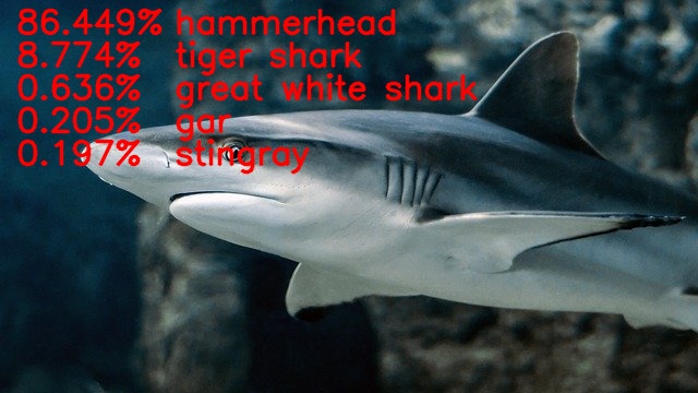
Here, the prediction seems a bit wrong. Although the image is that of a shark, it is not a hammerhead for sure. The next prediction, that is, tiger shark might be more appropriate.

From all the above cases, we can infer one thing. The EfficientNetB0 prediction is very fast, even on a CPU. Now let’s try out the prediction on a GPU. These are going to be a similar set of commands, just with --device cuda.

python efficientnet_classification.py --input input/image_1.jpg --device cuda

Computation device: cuda
sports car 0.5630043148994446
convertible 0.2391492873430252
grille 0.04134492576122284
racer 0.03619944304227829
car wheel 0.01730671152472496
Forward pass time: 1.283 seconds

python efficientnet_classification.py --input input/image_2.jpg --device cuda

Computation device: cuda
French bulldog 0.9024390578269958
Boston bull 0.022948967292904854
Staffordshire bullterrier 0.0032272031530737877
boxer 0.001872420310974121
Cardigan 0.0011130491038784385
Forward pass time: 0.431 seconds

python efficientnet_classification.py --input input/image_3.jpg --device cuda

Computation device: cuda
hammerhead 0.8640864491462708
tiger shark 0.08800099790096283
great white shark 0.0063613704405725
gar 0.002056644530966878
stingray 0.0019733444787561893
Forward pass time: 0.430 seconds

In the first case, the GPU took more than one second. And in the next two images, it took almost half a second for the forward pass. This is mostly because GPUs perform best when we try to utilize them to the full extent or continuously. This means that pass input tensors in batches, or one after the other really quickly.

Let’s try the second option in the next section while at the same time trying to compare the forward pass time with the ResNet50 model.

Comparing Forward Pass Times of EfficientNetB0 and ResNet50

This is the final coding section of the post. Here, we will write the script to compare the forward pass times of EfficientNetB0 and the ResNet50 model.

But why compare with ResNet50?

The main reason is the accuracy. Although EfficientNetB0 has only 5.3 million parameters compared to the 26 million parameters of ResNet50, they are in the same accuracy range. In fact, EfficientNetB0 is slightly ahead with 77.1% top-1 accuracy compared to the 76% top-1 accuracy of ResNet50. In the EfficientNet paper, the authors also compare the different EfficientNet models in a similar manner.

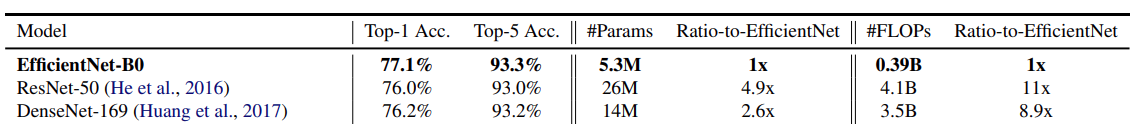
You can find all the comparisons in Table 2 of the EfficientNet paper.

All the code here will go into the compare.py script.

Starting with the imports and constructing the argument parser.

import cv2
import argparse

from utils import (
    load_efficientnet_model, preprocess, 
    read_classes, run_through_model, load_resnet50_model,
    plot_time_vs_iter
)

# Construct the argumet parser to parse the command line arguments.
parser = argparse.ArgumentParser()
parser.add_argument('-i', '--input', default='input/image_1.jpg', 
                    help='path to the input image')
parser.add_argument('-d', '--device', default='cpu', 
                    help='computation device to use', 
                    choices=['cpu', 'cuda'])
args = vars(parser.parse_args())

We need the run_through_model, load_resnet50_model, and plot_time_vs_iter functions from the utils module this time.

The argument parser is the same as the previous script.

Define Constants and Forward Pass Through the Models

Let’s define a few constants that we need along with executing the necessary helper functions.

# Number of times to forward pass through the model.
N_RUNS = 500
# Set the computation device.
DEVICE = args['device']
# Load the ImageNet class names.
categories = read_classes()
# Initialize the image transforms.
transform = preprocess()

print(f"Computation device: {DEVICE}")

We are defining N_RUNS = 500 indicating that we will propagate the input image 500 times through each model. The other parts remain similar to the EfficientNetB0 classification code.

Next, let’s read and preprocess the image. Along with that, we will feed the input image to each of the models, and plot the time vs iteration graph.

image = cv2.imread(args['input'])
rgb_image = cv2.cvtColor(image, cv2.COLOR_BGR2RGB)
# Apply transforms to the input image.
input_tensor = transform(image)
# Add the batch dimension.
input_batch = input_tensor.unsqueeze(0)
# Move the input tensor and model to the computation device.
input_batch = input_batch.to(DEVICE)

# Initialize the EfficientNetB0 model model.
model = load_efficientnet_model()
model.to(DEVICE)
print('Running through EfficinetNetB0 model.')
effcientnetb0_times = run_through_model(model, input_batch, N_RUNS)

# Initialize the ResNet50 model model.
model = load_resnet50_model()
model.to(DEVICE)
print('Running through ResNet50 model.')
resnet50_times = run_through_model(model, input_batch, N_RUNS)

plot_time_vs_iter(
    model_names=['EfficientNetB0', 'ResNet50'],
    time_lists=[effcientnetb0_times, resnet50_times],
    device=DEVICE
)

On lines 41 and 47, we are feeding the input to EfficientNetB0 and ResNet50 models. The run_through_model() function will run the input through the model 500 times. It will print the average time taken and return a list containing the forward pass time for each iteration.

Finally, starting from line 40, we plot the time vs iteration graph.

This completes all the code that we need. Now we can execute the script.

Executing compare.py

For the execution part, we will first use the CPU as the computation device, then the GPU.

Starting with the CPU execution.

python compare.py --device cpu

The following is the output on the terminal.

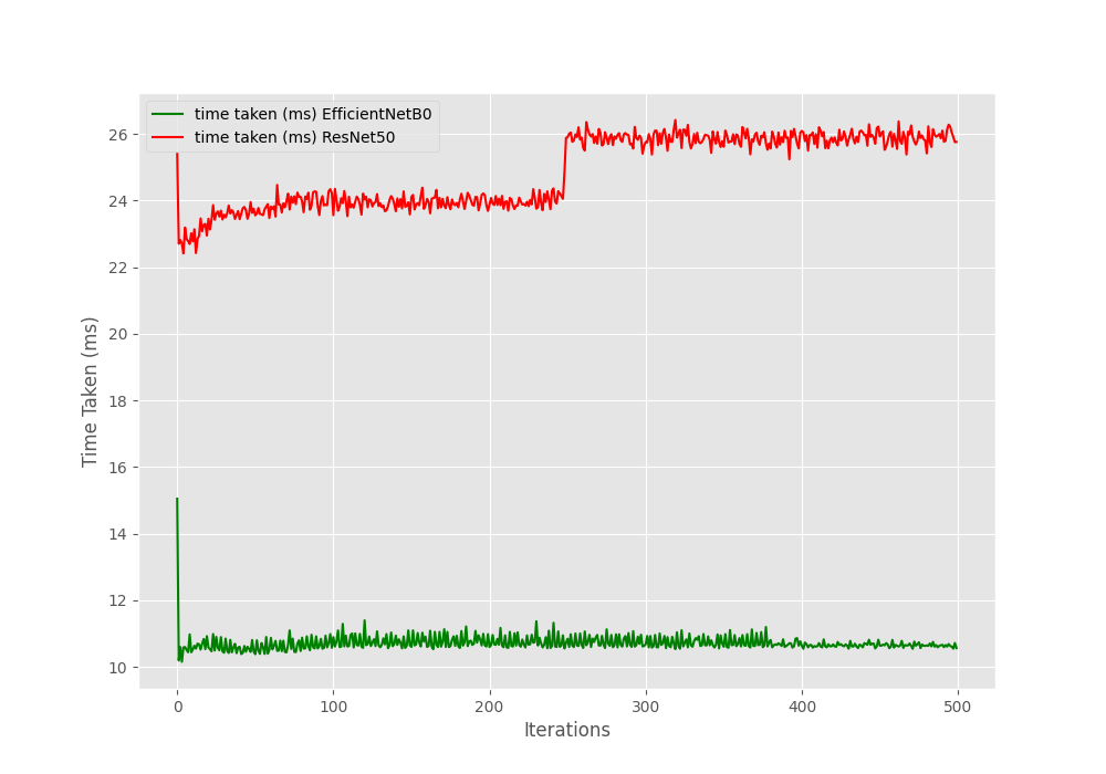
Computation device: cpu
Running through EfficinetNetB0 model.
10.721 milliseconds

Running through ResNet50 model.
24.861 milliseconds

The EffcientNetB0 model is taking around 10.721 milliseconds on average which is less than half the time compared to the ResNet50 model. Looks like the EfficientNetB0 model is much faster.

Next, we will execute the same code with GPU as the computation device. Now, if you remember, when inferencing on a single image, the GPU computation time was higher than that of CPU. Let’s see what happens in the case of GPU.

python compare.py --device cuda

Computation device: cuda
Running through EfficinetNetB0 model.
7.031 milliseconds

Running through ResNet50 model.
4.932 milliseconds

The average run time was surely reduced. But we can see something very interesting. This time, the EfficientNetB0 model was around 2 milliseconds slower than ResNet50.

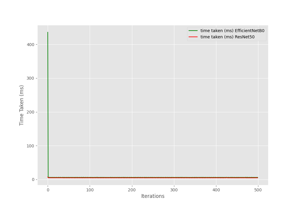
This might be because of the MBConv layers which are the main building blocks of EfficientNet. This repository also shows similar results. Although the inference times are a bit different because of differences in platform and hardware.

In future posts, we will carry out transfer learning and fine tuning to show the real power of EfficientNets.

Summary and Conclusion

In this post, we carried out image classification inference using PyTorch pretrained Efficient model. We used the EfficientNetB0 model here. Then we also saw the inference time comparison between EfficientNetB0 and ResNet50 on both CPU and GPU. I hope that this post was helpful to you.

If you have any doubts, thoughts, or suggestions, please leave them in the comment section. I will surely address them.

You can contact me using the Contact section. You can also find me on LinkedIn, and Twitter.