
FasterViT is a family of Vision Transformer models that is both fast and provides better accuracy than other ViT models. It combines the local representation learning of CNNs and the global learning properties of ViTs. In this article, we will cover the FasterViT model for image classification.

We will go through image inference using the pretrained network along with a brief of its architectural components. Furthermore, we will also fine-tune a FasterViT model for image classification.
We will cover the following topics in this article
- We will start with a discussion about the contributions of the FasterViT paper, the architecture, and the results.
- Next, we will use a pretrained FasterViT model for running inference on images.
- Then, we will fine-tune the FasterViT model to recognize cotton disease.
FasterViT for Computer Vision Tasks
The FasterViT model was introduced by researchers at NVIDIA. It is a hybrid model containing both, the features of CNN and that of Vision Transformers.
In this section, we will briefly cover the issues of previous ViT models, the contributions of FasterViT, and some of the results from the paper.
Limitations of Previous ViT Models
Most of the previous ViT architectures (including the first Vision Transformer model) have an isotropic architecture. This means that the model uses the same feature resolution throughout the network without any downsampling.
However, it is observed that for fine-grained computer vision tasks like object detection, and semantic segmentation, using multi-scale features yields better results.
Swin Transformer mitigates this issue to some extent by introducing windowed attention for multi-scale features. However, local attention with small windows can lead to the loss of local features. Especially, when the input resolution is too high. Furthermore, the Swin Transformer model’s throughput becomes too low for larger resolutions.
For this, the FasterViT model introduces several new features and contributions.
Features and Contributions of the FasterViT Model
Here are some of the major features and contributions of the Faster ViT paper.
- It is a hybrid model combining the benefits of the spatial induction bias of CNNs and the global modeling features of the attention mechanism.
- This hybrid architecture allows FasterViT to scale effectively for high resolution images.
- The paper also introduces the Hierarchical Attention module (HAT). It helps in capturing the cross-window interactions of local regions and long-rage spatial dependencies.
- The FasterViT model is also competitive when tuned for fine-grained tasks like object detection and semantic segmentation.
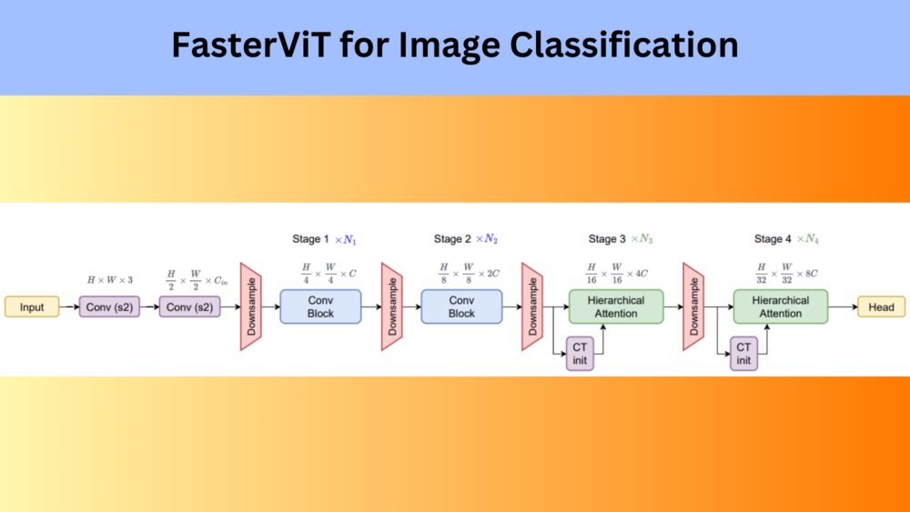
The FasterViT Architecture
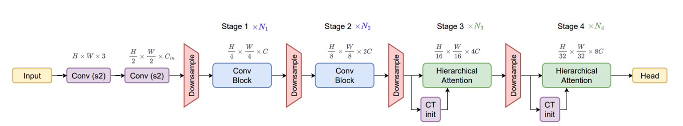
As discussed earlier, FasterViT combines CNN blocks and the attention mechanism of Transformers.
The above figure shows the general architecture of the FasterViT model. FasterViT contains four stages.
- The first two contain the CNN and downsampling blocks which help in reducing the feature map resolution. At the same time, the number of channels keeps on doubling at each stage.
- The third and fourth stages contain the Hierarchical Attention module. Essentially, this is where the attention mechanism of the model kicks in.
We can also notice that the final feature map resolution is downsampled by 32 times relative to the original image. After that, the model contains the final head. This head can be a classification head, segmentation head, or even a modified head for object detection.
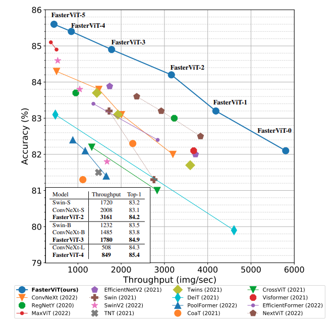
ImageNet1K Result Comparison
As we will only carry out image classification experiments in this article, we will cover the results for ImageNet1K only.
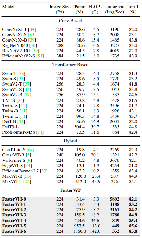
As we can see, the FasterViT model beats all other models in terms of throughput and accuracy when compared on a scale of the number of parameters.
This shows the efficacy of the FasterViT models for image classification.
Next, we will focus on the coding section where we will use the FasterViT model for image classification inference and fine-tuning.
Project Directory Structure
Let’s take a look at the directory structure of the project.
├── input
│   ├── cotton_disease_inference_data
│   ├── Cotton-Disease-Training
│   ├── Cotton-Disease-Validation
│   ├── Customized Cotton Dataset-Complete
│   └── inference_images
├── outputs
│   ├── inference_results
│   ├── accuracy.png
│   ├── aphids.jpg
│   ├── best_model.pth
│   ├── image_1.jpg
│   ├── image_2.jpg
│   ├── loss.png
│   └── model.pth
├── weights
│   └── fastervit_0_224_1k.pth.tar
├── datasets.py
├── imagenet_classes.txt
├── inference.py
├── model.py
├── pretrained_inference.py
├── requirements.txt
├── train.py
└── utils.py
- The
inputdirectory contains the training dataset and inference data as well. We will discuss more about the training dataset in the fine-tuning FasterViT section. - The
outputsdirectory contains the pretrained image inference outputs as well as outputs from the fine-tuning process. - We also have a
weightsdirectory where the pretrained FasterViT model weight file is present. - Directly inside the parent project directory, we have all the code files. It also contains a
requirements.txtfile for easier installation of all the major dependencies.
Installing FasterViT Library
If you have all other requirements installed, then you can install just the FasterViT library using the following command.
pip install fastervit
All the code files, pretrained weights, and inference data will be provided along with the downloadable zip file. If you intend to run the training process, please download the training data as per the description from the dataset discussion section further below.
Download Code
Running Inference using Pretrained FasterViT
The FasterViT repository contains the links to all the pretrained models. It provides the weights to 7 different scales of FasterViT models pretrained on the ImageNet1K dataset:
- FasterViT-0
- FasterViT-1
- FasterViT-2
- FasterViT-3
- FasterViT-4
- FasterViT-5
- FasterViT-6
We will use the pretrained FasterViT-0 for inference and later for fine-tuning. This model contains 34.1 million parameters.
The downloadable zip file already contains the pretrained weight. You can also find the link in this table.
Let’s start with the coding part. The code for running image inference using the pretrained FasterViT-0 model is in the pretrained_inference.py file.
The following code block contains the import statements and the construction of the argument parser.
from fastervit import create_model

import cv2
import torch
import argparse
import time
import os

parser = argparse.ArgumentParser()
parser.add_argument(
    '--input',
    help='path to the input image',
    default='input/inference_images/image_1.jpg'
)
parser.add_argument(
    '--weights',
    help='path to the pretrained weights file',
    default='weights/fastervit_0_224_1k.pth.tar'
)
parser.add_argument(
    '--classes-txt',
    help='path to the text file containing class names',
    default='imagenet_classes.txt',
    dest='classes_txt'
)
args = parser.parse_args()
We import the create_model function from the fastervit module that we will later use for initializing the pretrained model.
Among the argument parser, we have the following flags:
--input: The path to the input image.--weights: The path to the pretrained weight file. It defaults to the weight file inside theweightsdirectory.--classes-txt: This is the path to the image text file containing the ImageNet1K classes.
Next, we create the outputs directory and initialize the pretrained FasterViT model.
os.makedirs('outputs', exist_ok=True)

with open(args.classes_txt, 'r') as f:
    categories = [s.strip() for s in f.readlines()]

model = create_model(
    'faster_vit_0_224',
    pretrained=True,
    model_path='weights/fastervit_0_224_1k.pth.tar'
).eval()
The create_model function accepts the three mandatory arguments:
- The name of the model.
- Whether we want to load the pretrained weights or not.
- And the path to the pretrained weights.
Along with that, we also read the ImageNet1K class text file.
Then, we read the image and forward pass it through the model.
image = cv2.imread(args.input)
orig_image = image.copy()
image = cv2.cvtColor(image, cv2.COLOR_BGR2RGB)
image = cv2.resize(image, (224, 224))

image = torch.tensor(image, dtype=torch.float).permute(2, 0, 1).unsqueeze(0)

start_time = time.time()

with torch.no_grad():
    outputs = model(image)

end_time = time.time()

# Get the softmax probabilities.
probabilities = torch.nn.functional.softmax(outputs[0], dim=0)

# Check the top 5 categories that are predicted.
top5_prob, top5_catid = torch.topk(probabilities, 5)
for i in range(top5_prob.size(0)):
    cv2.putText(orig_image, f"{top5_prob[i].item()*100:.3f}%", (15, (i+1)*30),
                cv2.FONT_HERSHEY_SIMPLEX,
                1, (0, 0, 255), 2, cv2.LINE_AA)
    cv2.putText(orig_image, f"{categories[top5_catid[i]]}", (160, (i+1)*30),
                cv2.FONT_HERSHEY_SIMPLEX,
                1, (0, 0, 255), 2, cv2.LINE_AA)
    print(categories[top5_catid[i]], top5_prob[i].item())
cv2.imshow('Result', orig_image)
cv2.waitKey(0)

# Define the outfile file name.
save_name = f"outputs/{args.input.split('/')[-1].split('.')[0]}.jpg"
cv2.imwrite(save_name, orig_image)
print(f"Forward pass time: {(end_time-start_time):.3f} seconds")
After getting the logits, we calculate the softmax probabilities and annotate the top-5 predictions on the image.
Executing Pretrained Image Inference
Let’s run inference using the default arguments and check the results.
python pretrained_inference.py
We get the following result.
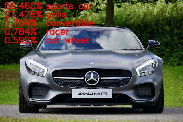
The model predicts the top-class as a sports car with more than 56% accuracy.
Let’s try with a different image now.
python pretrained_inference.py --input input/inference_images/image_2.jpg
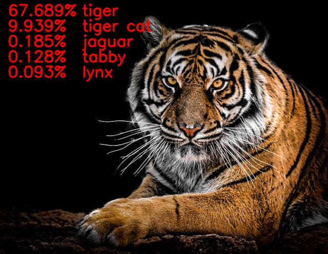
This time also, the model is able is predict the top-class as a tiger with more than 67% accuracy. Looks like our pretrained inference approach is correct.
Fine Tuning FasterViT for Cotton Disease Classification
Fine tuning the FasterViT model is no more different than fine tuning any other Vision Transformer model. The only part that changes is the model preparation.
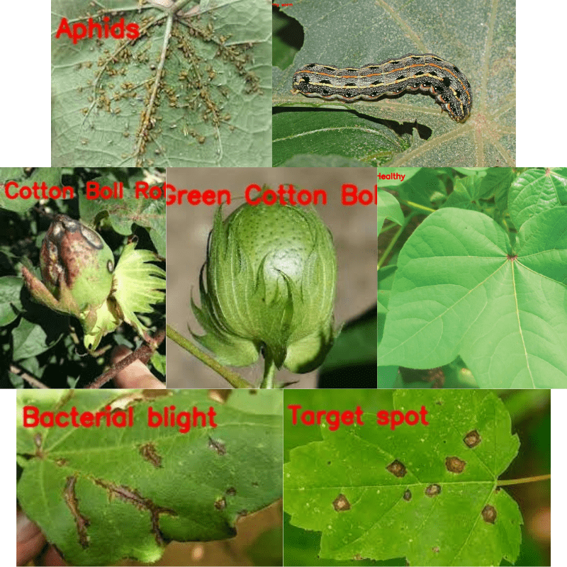
However, before that, let’s discuss the dataset a bit. We will use a cotton disease classification dataset containing 8 classes. They are:
- Aphids
- Army worm
- Bacterial blight
- Cotton Boll Rot
- Green Cotton Boll
- Healthy
- Powdery mildew
- Target spot
Downloading and extracting the dataset will show the following structure.
├── Cotton-Disease-Training
│   └── trainning
│       └── Cotton leaves - Training
│           └── 800 Images
│               ├── Aphids
│               ├── Army worm
│               ├── Bacterial blight
│               ├── Cotton Boll Rot
│               ├── Green Cotton Boll
│               ├── Healthy
│               ├── Powdery mildew
│               └── Target spot
├── Cotton-Disease-Validation
│   └── validation
│       └── Cotton plant disease-Validation
│           └── Cotton plant disease-Validation
│               ├── Aphids edited
│               ├── Army worm edited
│               ├── Bacterial Blight edited
│               ├── Cotton Boll rot
│               ├── Green Cotton Boll
│               ├── Healthy leaf edited
│               ├── Powdery Mildew Edited
│               └── Target spot edited
└── Customized Cotton Dataset-Complete
    └── content
        ├── trainning
        │   └── Cotton leaves - Training
        │       └── 800 Images
        └── validation
            └── Cotton plant disease-Validation
                └── Cotton plant disease-Validation
We will use the Cotton-Disease-Training and Cotton-Disease-Validation directories for our purpose.
Here are some examples from the dataset.
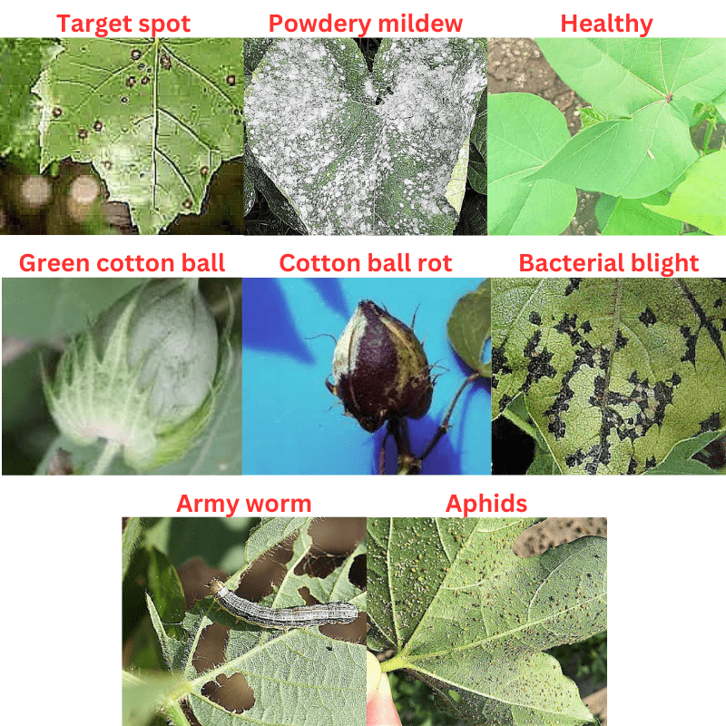
We will not go through all the coding details here. Mostly, we will cover the model preparation as other parts of the code are similar to any other PyTorch image classification problem. Feel free to take a look at the code in detail after downloading and extracting the zip file.
Preparing the FasterViT Model for Fine Tuning
The model preparation code is present in the model.py file. Following are the contents of the file.
from fastervit import create_model

import torch.nn as nn

def build_model(num_classes=10):
    model = create_model(
        'faster_vit_0_224',
        pretrained=True,
        model_path='weights/fastervit_0_224_1k.pth.tar'
    )

    model.head = nn.Linear(in_features=512, out_features=num_classes, bias=True)

    return model

if __name__ == '__main__':
    model = build_model()
    print(model)
    # Total parameters and trainable parameters.
    total_params = sum(p.numel() for p in model.parameters())
    print(f"{total_params:,} total parameters.")
    total_trainable_params = sum(
        p.numel() for p in model.parameters() if p.requires_grad)
    print(f"{total_trainable_params:,} training parameters.")
We initialize the model in the same manner as we did for pretrained image inference. Following that, we also modify the final classification layer so that the output features correspond to the number of classes in the dataset.
Dataset and Training Parameters
Here are some additional details regarding the dataset preparation:
- We are resizing both, the training and validation set images to 224×224 resolution.
- The datasets go through the ImageNet normalization as we are using an ImageNet pretrained model.
- Additionally, the training dataset goes through flipping, rotation, and sharpness augmentation using PyTorch transforms.
Here are the training hyperparameters and settings:
- We use the Adam optimizer.
- A Multi-Step learning rate scheduler is employed to reduce the learning rate by a factor of after 5 epochs.
- The best model is saved whenever the validation loss is lower than the previous least one.
Running the FasterViT Fine Tuning Experiment
The following fine tuning experiments were run on a machine with 10GB RTX 3080 GPU, 10th generation i7 CPU, and 32 GB of RAM.
We can start the FasterViT fine tuning process by executing the following command.
python train.py -lr 0.0001 --epochs 10 --batch 16
We are training the model for 10 epochs with an initial learning rate of 0.0001 and a batch size of 16.
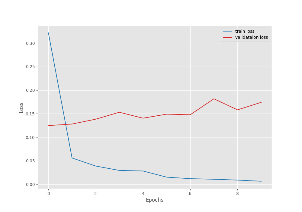
Here are the results.
[INFO]: Epoch 1 of 10
Training
100%|████████████████████████████████████████████████████████████████████████████████████████████████████████████████████████████████████████████████████████████████████████████| 415/415 [00:25<00:00, 16.22it/s]
Validation
100%|██████████████████████████████████████████████████████████████████████████████████████████████████████████████████████████████████████████████████████████████████████████████| 23/23 [00:00<00:00, 23.40it/s]
Training loss: 0.322, training acc: 91.762
Validation loss: 0.125, validation acc: 97.199

Best validation loss: 0.1247152074078179

Saving best model for epoch: 1

--------------------------------------------------
Adjusting learning rate of group 0 to 1.0000e-04.
[INFO]: Epoch 2 of 10
Training
100%|████████████████████████████████████████████████████████████████████████████████████████████████████████████████████████████████████████████████████████████████████████████| 415/415 [00:23<00:00, 17.48it/s]
Validation
100%|██████████████████████████████████████████████████████████████████████████████████████████████████████████████████████████████████████████████████████████████████████████████| 23/23 [00:00<00:00, 26.35it/s]
Training loss: 0.056, training acc: 98.310
Validation loss: 0.128, validation acc: 97.759
--------------------------------------------------
.
.
.
Adjusting learning rate of group 0 to 1.0000e-05.
[INFO]: Epoch 10 of 10
Training
100%|████████████████████████████████████████████████████████████████████████████████████████████████████████████████████████████████████████████████████████████████████████████| 415/415 [00:23<00:00, 17.56it/s]
Validation
100%|██████████████████████████████████████████████████████████████████████████████████████████████████████████████████████████████████████████████████████████████████████████████| 23/23 [00:00<00:00, 25.53it/s]
Training loss: 0.006, training acc: 99.834
Validation loss: 0.174, validation acc: 97.199
--------------------------------------------------
Adjusting learning rate of group 0 to 1.0000e-05.
TRAINING COMPLETE
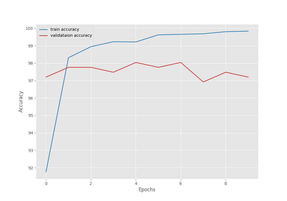
Interestingly, even with a lower starting learning rate and a learning rate scheduler, the validation loss does not improve after the first epoch.
The best validation loss is 0.124 with a corresponding validation accuracy of 97.19%.
Following are the accuracy and loss graphs.
Inference using the Fine Tuned Faster ViT Model
Now, we can use the inference.py script to run inference on the image present in the input/cotton_disease_inference_data directory. There is one image from each class.
python inference.py
Interestingly, the model can predict each class correctly.
Of course, if we have more images from each class the model is bound to make a mistake as it reached only 97% validation accuracy. Nonetheless, it is extremely interesting to note how well the model performs with limited data and just a few epochs of fine-tuning.
Summary and Conclusion
In this article, we covered the FasterViT model for image classification. Starting with a brief on the model architecture, to pretrained image classification, and fine-tuning, we covered a lot. In later articles, we will cover FasterViT for object detection and semantic segmentation. I hope that this article was worth your time.
If you have any doubts, thoughts, or suggestions, please leave them in the comment section. I will surely address them.
You can contact me using the Contact section. You can also find me on LinkedIn, and X.

4 thoughts on “FasterViT for Image Classification”