
In this article, we will modify the FasterViT model for semantic segmentation.
FasterViT is a family of CNN-Transformer hybrid models for deep learning based computer vision tasks. The FasterViT models are faster and more accurate on several computer vision benchmarks, particularly the ImageNet dataset. We can also modify the model for semantic segmentation to get excellent results on a custom dataset. Although it is not straightforward and requires several changes to the architecture, it is possible. In this article, we will cover the architectural details and the changes we must make to the FasterViT model for semantic segmentation.
We will cover the following topics in this article
- We will start with a short discussion of the dataset for training the FasterViT segmentation model.
- Next, we will move to the coding section where:
- First, we will cover the architectural changes to the FasterViT model.
- Second, we will discuss the major parts of the dataset preparation steps and the hyperparameter settings.
- Third, we will train the model and observe the results.
- Finally, we will use the trained FasterViT segmentation model to run inference on images and videos.
Note: Majorly, this article will cover the architectural changes that are needed in the FasterViT model to convert it into a performant semantic segmentation model. We will skip over other parts of the code to some extent. However, the entire codebase is downloadable.
If you are new to FasterViT, be sure to check out the previous article, where we covered FasterViT for image classification. In the article:
- We begin with the paper and FasterViT architecture discussion.
- Next, using the pretrained FasterViT model for image classification.
- Then, fine-tuning the model on a custom image classification dataset.
Let’s jump into the article now.
The Leaf Disease Segmentation Dataset
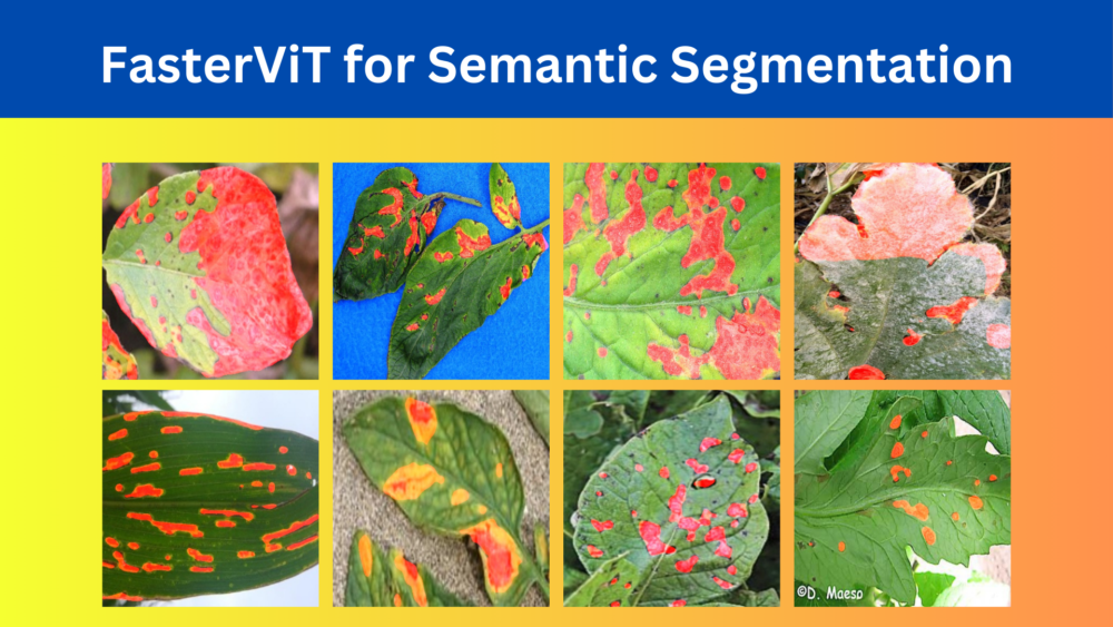
We will use the leaf disease segmentation dataset in this article to train the FasterViT based semantic segmentation model.
Although a binary segmentation dataset, it is challenging enough because of the diversity in shapes and sizes of the segmentation map. The dataset consists of segmentation maps for various types of plant leaf diseases.
After downloading and extracting the dataset from Kaggle, you will find the following directory structure.
leaf_disease_segmentation/
├── aug_data
│   ├── train_images
│   ├── train_masks
│   ├── valid_images
│   └── valid_masks
└── orig_data
    ├── train_images
    ├── train_masks
    ├── valid_images
    └── valid_masks
There are two subfolders, one with the augmented data and one with the original data. As we will apply our own augmentations, so, we will use the data in the orig_data directory. This in turn contains subfolders for images and masks with a training and a validation split. There are 498 training and 90 validation samples.
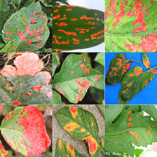
Here are a few samples from the training set.
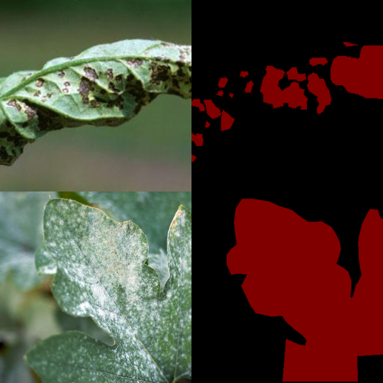
As we can see, segmentation maps can vary from large patches to even small dots on some of the leaves. This makes it an interesting dataset to test any new segmentation model. As the dataset is not too large, the training also won’t take long.
If you are interested in knowing how other models perform on this dataset, you will find the following articles interesting:
Project Directory Structure
Let’s take a look at the project directory structure.
├── input
│   ├── inference_data
│   │   ├── video_1.mp4
│   │   └── video_1_trimmed.mp4
│   └── leaf_disease_segmentation
│       ├── aug_data
│       └── orig_data
├── outputs
│   ├── inference_results_image [90 entries exceeds filelimit, not opening dir]
│   ├── inference_results_video
│   │   ├── video_1_trimmed.mp4
│   │   └── video_2_trimmed.mp4
│   ├── valid_preds [50 entries exceeds filelimit, not opening dir]
│   ├── accuracy.png
│   ├── best_model_iou.pth
│   ├── best_model_loss.pth
│   ├── loss.png
│   ├── miou.png
│   └── model.pth
├── weights
│   └── faster_vit_0.pth.tar
├── config.py
├── datasets.py
├── engine.py
├── inference_image.py
├── inference_video.py
├── metrics.py
├── segmentation_model.py
├── train.py
└── utils.py
- The
inputdirectory contains the training data that we observed in the previous section. It also contains the inference data. - In the
outputsdirectory, we have the results from the training as well as the inference runs. - The
weightsdirectory contains the FasterViT ImageNet pretrained weights. - In the parent directory, we have several Python code files. Among these, we will explore the
segmentation_model.py.
All the code files, pretrained weights, and inference data will be provided along with the downloadable zip file. If you intend to run the training process, please download the training data as per the description from the dataset discussion section further below.
Download Code
Major Dependencies
Here are the major libraries that we need for the code in this article to run:
- timm (Torch Image Models)
- fastervit
- albumentations
- PyTorach and Torchvision
You can install all of these using the requirements.txt file that comes along with the code base.
pip install -r requirements.txt
We are done with all the setup that we need to move ahead with semantic segmentation using FasterViT.
FasterViT for Semantic Segmentation
Let’s now focus on the coding part of converting the FasterViT ImageNet pretrained model into a semantic segmentation model.
Converting the FasterViT Image Classification Model to a Semantic Segmentation Model
The entire code for the model architecture is present in the segmentation_model.py.
Before we move ahead with exploring the code, a bit of background first. The FasterViT library provides two sets of model architectures. One is the original architecture meant for image classification which can only deal with fixed resolution images. The other one is a modified architecture that we can initialize with any image resolution of our choice. This is the architecture that we will use here. In fact, among the 7 different scales of architecture, we will use the smallest one, FasterViT-0.
Although the entire library is pip installable, the segmentation_model.py file contains the original code from the repository (fastervit_any_res.py). We further modify this code to make it semantic segmentation compliant. There are two primary reasons for this:
- The original architecture contains several nested module lists. This makes it difficult to extract multi-level convolution features just by initializing the model through the API and trying to traverse it.
- Having the entire original code makes it way easier to introduce our custom segmentation head and different processing steps in between. We will get to see the details in the following section.
The FasterViT Class
The entire model architecture is quite big. Our main focus here is the FasterViT class. This is the final class that gets initialized while loading the model. This is also the class where the image classification head is present. We will discard this head in the forward pass and introduce our custom segmentation head for semantic segmentation.
Let’s check the class and its __init__ method.
class FasterViT(nn.Module):
    """
    FasterViT based on: "Hatamizadeh et al.,
    FasterViT: Fast Vision Transformers with Hierarchical Attention
    """

    def __init__(self,
                 dim,
                 in_dim,
                 depths,
                 window_size,
                 ct_size,
                 mlp_ratio,
                 num_heads,
                 resolution=[224, 224],
                 drop_path_rate=0.2,
                 in_chans=3,
                 num_classes=1000,
                 qkv_bias=True,
                 qk_scale=None,
                 drop_rate=0.,
                 attn_drop_rate=0.,
                 layer_scale=None,
                 layer_scale_conv=None,
                 layer_norm_last=False,
                 hat=[False, False, True, False],
                 do_propagation=False,
                 **kwargs):
        """
        Args:
            dim: feature size dimension.
            in_dim: inner-plane feature size dimension.
            depths: layer depth.
            window_size: window size.
            ct_size: spatial dimension of carrier token local window.
            mlp_ratio: MLP ratio.
            num_heads: number of attention head.
            resolution: image resolution.
            drop_path_rate: drop path rate.
            in_chans: input channel dimension.
            num_classes: number of classes.
            qkv_bias: bool argument for query, key, value learnable bias.
            qk_scale: bool argument to scaling query, key.
            drop_rate: dropout rate.
            attn_drop_rate: attention dropout rate.
            layer_scale: layer scale coefficient.
            layer_scale_conv: conv layer scale coefficient.
            layer_norm_last: last stage layer norm flag.
            hat: hierarchical attention flag.
            do_propagation: enable carrier token propagation.
        """
        super().__init__()
        if type(resolution)!=tuple and type(resolution)!=list:
            resolution = [resolution, resolution]
        num_features = int(dim * 2 ** (len(depths) - 1))
        self.num_classes = num_classes
        self.patch_embed = PatchEmbed(in_chans=in_chans, in_dim=in_dim, dim=dim)
        dpr = [x.item() for x in torch.linspace(0, drop_path_rate, sum(depths))]
        self.levels = nn.ModuleList()
        if hat is None: hat = [True, ]*len(depths)
        for i in range(len(depths)):
            conv = True if (i == 0 or i == 1) else False
            level = FasterViTLayer(dim=int(dim * 2 ** i),
                                   depth=depths[i],
                                   num_heads=num_heads[i],
                                   window_size=window_size[i],
                                   ct_size=ct_size,
                                   mlp_ratio=mlp_ratio,
                                   qkv_bias=qkv_bias,
                                   qk_scale=qk_scale,
                                   conv=conv,
                                   drop=drop_rate,
                                   attn_drop=attn_drop_rate,
                                   drop_path=dpr[sum(depths[:i]):sum(depths[:i + 1])],
                                   downsample=(i < 3),
                                   layer_scale=layer_scale,
                                   layer_scale_conv=layer_scale_conv,
                                   input_resolution=[int(2 ** (-2 - i) * resolution[0]),
                                                     int(2 ** (-2 - i) * resolution[1])],
                                   only_local=not hat[i],
                                   do_propagation=do_propagation)
            self.levels.append(level)
        self.norm = LayerNorm2d(num_features) if layer_norm_last else nn.BatchNorm2d(num_features)
        self.avgpool = nn.AdaptiveAvgPool2d(1)
        self.head = nn.Linear(num_features, num_classes) if num_classes > 0 else nn.Identity()
        self.apply(self._init_weights)

        # Additional convolutional layers.
        self.upsample_and_classify = nn.Sequential(
                # Convolutional layers for feature refinement can be added here
                nn.Conv2d(2048, 768, kernel_size=3, padding=1),
                nn.GroupNorm(8, 768),
                nn.ReLU(),

                nn.Conv2d(768, 1024, kernel_size=3, padding=1),
                nn.GroupNorm(8, 1024),
                nn.ReLU(),

                nn.Conv2d(1024, 768, kernel_size=3, padding=1),
                nn.GroupNorm(8, 768),
                nn.ReLU(),

                nn.Conv2d(768, 512, kernel_size=3, padding=1),
                nn.GroupNorm(8, 512),
                nn.ReLU(),

                nn.Upsample(size=resolution, mode='bilinear', align_corners=False),
                nn.Conv2d(512, self.num_classes, kernel_size=1)
            )

        # Addition Conv2d blocks to match the output channels for multi-level
        # featues before concatenation.
        self.conv2d_block1 = nn.Conv2d(in_channels=128, out_channels=512, kernel_size=3)
        self.conv2d_block2 = nn.Conv2d(in_channels=256, out_channels=512, kernel_size=3)

        # Upsampling layer to match the spatial dimension of multi-level features.
        self.upsample = nn.Upsample(size=(128, 128), mode='bilinear', align_corners=False)
We can see several initializations in the above method along with the self.head meant for image classification.
The additional convolutional layers for semantic segmentation starts from line 89 in the above code block. The self.upsample_and_classify introduces a Sequential segmentation head. We can also see a series of Conv2d, GroupNorm, and ReLU before the final upsampling and segmentation layer. The motivation for this comes from here where the authors of FasterViT repository introduce a segmentation head for DINO segmentation.
Furthermore, remember that the original FasterViT architecture has several stages of 2D convolutional downsampling.
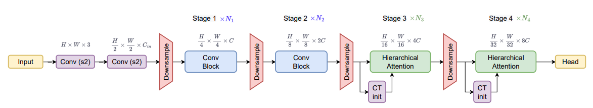
As we will be extracting those multi-level features and trying to concatenate them, we need some way to match the spatial resolution. That’s what the self.upsample does. It will bring all the multi-level features to a spatial resolution of 128×128. Along with that, we also match the output channels of the two multi-level features to 512 as we can see in self.conv2d_block1 and self.conv2d_block2.
The FasterViT Semantic Segmentation Forward Passes
Let’s take a look at the forward passes of the modified FasterViT Semantic Segmentation model to make the process even clearer.
def forward_features(self, x):
        # Create a list to store the convolution features from each level.
        conv_features = []
        x = self.patch_embed(x)
        for level in self.levels:
            x = level(x)
            # Append each level's convolution feature.
            conv_features.append(x)
        x = self.norm(x)
        # Return both, the final output, and the convolution feature.
        return x, conv_features

    def forward(self, x):
        # Need only the forwarded features and not from the head part
        # that is meant for classification.
        x, conv_features = self.forward_features(x)

        # Extract all four level of convolution features.
        feature_1, feature_2, feature_3, feature_4 = conv_features

        # Get the unmatched output features to the same number for all four (check `__init__()`).
        feature_1 = self.conv2d_block1(feature_1)
        feature_2 = self.conv2d_block2(feature_2)

        # Upsample all four feature maps to the same spatial resolution (check `__init__()`).
        feature_1 = self.upsample(feature_1)
        feature_2 = self.upsample(feature_2)
        feature_3 = self.upsample(feature_3)
        feature_4 = self.upsample(feature_4)

        # Concatenate multi-level features.
        final_features = torch.cat([feature_1, feature_2, feature_3, feature_4], dim=1)

        # Finally, upsample and get the output segmentqation map.
        x = self.upsample_and_classify(final_features)

        return x
First comes the forward_features method. This extracts all the multi-level convolutional features. We have modified this to append all the multi-level features in the conv_features list and return it along with the final output.
Second, we have the final forward method. Originally, there was also a call to the classification head in this method which we have removed as we do not need that. First, we extract all the multi-level features on line19. Currently, the four of the features have the following shapes respectively.
- [1, 128, 64, 64]
- [1, 256, 32, 32]
- [1, 512, 16, 16]
- [1, 512, 16, 16]
So, first, we make the first two feature maps to have 512 output channels (lines 22 and 23). Then upsample each of the feature maps to 128×128 spatial resolution (lines 26 to 29). Next, we concatenate all features along the channel dimension which makes the final output dimension of 2048. This was the reason the final Sequential head was initialized with 2048 input channels.
Finally, we forward pass the concatenated features through the semantic segmentation head.
These are all the changes that we make to the FasterViT model to convert it to a semantic segmentation model. The final segmentation map will have the same shape as the input image resolution.
The Initialization Function
We will not be initializing the FasterViT class directly. Instead we have a faster_vit_0_any_res initialization function which accepts several keyword arguments.
def faster_vit_0_any_res(pretrained=False, **kwargs):
    depths = kwargs.pop("depths", [2, 3, 6, 5])
    num_heads = kwargs.pop("num_heads", [2, 4, 8, 16])
    window_size = kwargs.pop("window_size", [7, 7, 7, 7])
    ct_size = kwargs.pop("ct_size", 2)
    dim = kwargs.pop("dim", 64)
    in_dim = kwargs.pop("in_dim", 64)
    mlp_ratio = kwargs.pop("mlp_ratio", 4)
    resolution = kwargs.pop("resolution", [512, 512])
    drop_path_rate = kwargs.pop("drop_path_rate", 0.2)
    model_path = kwargs.pop("model_path", "weights/faster_vit_0.pth.tar")
    hat = kwargs.pop("hat", [False, False, True, False])

    pretrained_cfg = resolve_pretrained_cfg('faster_vit_0_any_res').to_dict()
    _update_default_kwargs(pretrained_cfg, kwargs, kwargs_filter=None)

    model = FasterViT(depths=depths,
                      num_heads=num_heads,
                      window_size=window_size,
                      ct_size=ct_size,
                      dim=dim,
                      in_dim=in_dim,
                      mlp_ratio=mlp_ratio,
                      resolution=resolution,
                      drop_path_rate=drop_path_rate,
                      hat=hat,
                      **kwargs)

    model.pretrained_cfg = pretrained_cfg
    model.default_cfg = model.pretrained_cfg
    if pretrained:
        if not Path(model_path).is_file():
            url = model.default_cfg['url']
            torch.hub.download_url_to_file(url=url, dst=model_path)
        model._load_state_dict(model_path)
    return model
Among the keyword arguments, the resolution one is the most important to specify the input image resolution.
Checking the Model with A Dummy Forward Pass
Now, let’s check the model with a dummy forward call.
if __name__ == '__main__':
    resolution = [512, 512]
    model = faster_vit_0_any_res(pretrained=True, resolution=resolution)
    model.upsample_and_classify[13] = nn.Conv2d(512, 2, kernel_size=(1, 1), stride=(1, 1))

    print(model)

    # Total parameters and trainable parameters.
    total_params = sum(p.numel() for p in model.parameters())
    print(f"{total_params:,} total parameters.")
    total_trainable_params = sum(
        p.numel() for p in model.parameters() if p.requires_grad)
    print(f"{total_trainable_params:,} training parameters.")

    randon_input = torch.randn((1, 3, *resolution))

    model.eval()
    with torch.no_grad():
        outputs = model(randon_input)

    print(outputs.shape)
After initializing the model, convert the final head with the number of classes in our dataset. This is important as the original model has 1000 output classes as it was a classification model originally.
We get the output as torch.Size([1, 2, 512, 512]) which is the same shape as the input image.
It is worthwhile to note that the final model contains 65 million parameters. It is quite large considering the original classification model had only 30 million parameters. However, as this is our first iteration of converting the model, we will first focus on getting the model to produce good results and then optimize it for fewer parameters.
This completes all the model related changes that we need to make to the FasterViT architecture to convert it to a semantic segmentation model.
Dataset Augmentation
The datasets.py file contains the preparation of the custom segmentation dataset and the data loaders.
We are applying the following image augmentations to the training dataset.
- Horizontal flipping
- Randomizing brightness and contrast
- Rotation
In addition to this, both, the training and validation samples (images and masks) are resized to 512×512 resolution during training. We can control the image resolution directly from the command line while training.
Training Hyperparameters and Settings
We are using the Adam optimizer for training the FasterViT semantic segmentation model. Two best models will be saved during training. One based on the least validation loss and another based on the highest mean IoU.
Furthermore, using the --scheduler command line argument we can tell the script whether to apply learning rate scheduling or not. For now, we are using a multi-step scheduling setting at epochs 25 and 30 to reduce the learning rate by a factor of 10.
Training the FasterViT Semantic Segmentation Model
The following training experiment was carried out on a machine with 10 GB RTX 3080 GPU, 10th generation i7 CPU, and 32 GB of RAM.
We can execute the following command to start the training.
python train.py --imgsz 512 512 --epochs 50 --lr 0.0001 --batch 2 --scheduler
We are training the model for 50 epochs, with an initial learning rate of 0.0001, a batch size of 2, and applying learning rate scheduling as well.
Here is the output from the terminal after 50 epochs.
EPOCH: 50
Training
100%|████████████████████| 249/249 [01:24<00:00,  2.95it/s]
Validating
100%|████████████████████| 45/45 [00:05<00:00,  7.98it/s]

Best validation IoU: 0.768908504523357

Saving best model for epoch: 50

Train Epoch Loss: 0.0606, Train Epoch PixAcc: 0.9703, Train Epoch mIOU: 0.884733
Valid Epoch Loss: 0.2014, Valid Epoch PixAcc: 0.9206 Valid Epoch mIOU: 0.768909
Adjusting learning rate of group 0 to 1.0000e-06.
--------------------------------------------------
TRAINING COMPLETE
We have the best validation IoU of 76.89%. We will use this model while running inference on images and videos.
Following are the mean IoU, pixel accuracy, and, loss graphs.
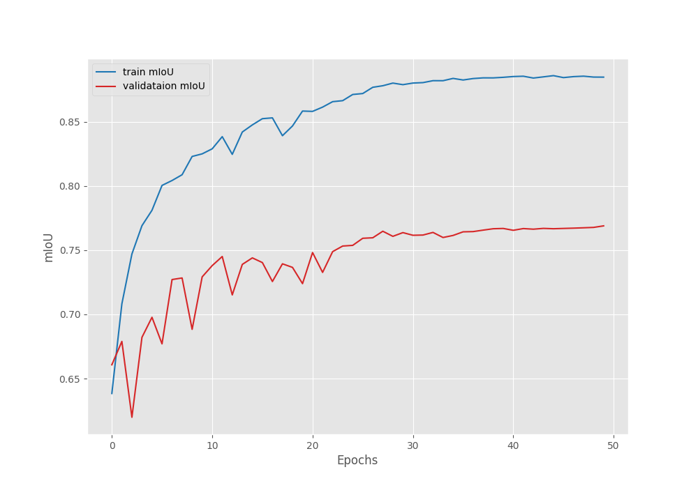
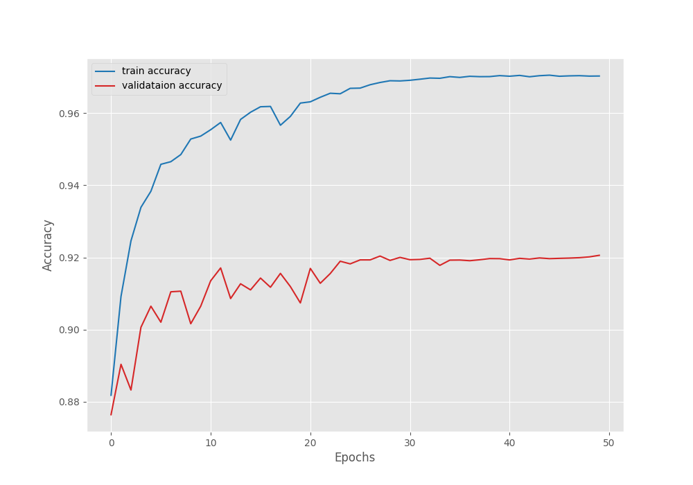
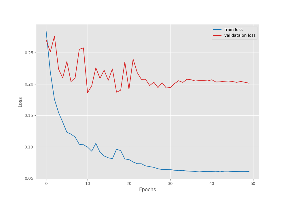
We can observe that the loss has again started to go down after epoch 41. So our decision to apply the learning rate scheduling was the correct. With this setting, we can train the model for a few more epochs.
Inference using the Trained FasterViT Segmentation Model on Validation Images
The inference_image.py script contains the code for running inference on a directory of images. Let’s run it and check the results.
python inference_image.py --imgsz 512 512 --input input/leaf_disease_segmentation/orig_data/valid_images/ --model outputs/best_model_iou.pth
We are providing the same image size as the model was trained on. Along with that, we also provide the path to the validation image directory and the best weights.
Here are some of the results.
The predicted segmentation maps are not bad at all, given that we are just using an ImageNet pretrained backbone and added our custom segmentation head.
Of course, there is room for improvement, which we will discuss later.
Inference on Videos using the Trained FasterViT Segmentation Model
Now, let’s try another inference experiment on a video from YouTube. For this, we use the inference_video.py script.
python inference_video.py --imgsz 512 512 --input input/inference_data/video_1_trimmed.mp4 --model outputs/best_model_iou.pth
Although not perfect, the model is certainly able to segment the diseased regions. The segmentation borders can be sharper. However, that is only possible with more optimization of the segmentation head, and our training techniques.
Takeaways
We obtained more than decent results after optimizing the FasterViT model for semantic segmentation just using a pretrained ImageNet backbone and added our segmentation head. We can still improve the results by pretraining the model on a large semantic segmentation dataset.
Furthermore, we can also use transposed convolution instead of upsampling in the segmentation head.
However, both of these are subject to several experimentations.
Summary and Conclusion
In this article, we modified the FasterViT model for semantic segmentation. We covered in detail how to change the forward pass of the original model with additional layers for segmentation. This included concatenating multi-level features, adding a new segmentation head, and optimizing the necessary parameters. We also obtained good results from the custom model. I hope that this article was worth your time.
If you have any doubts, thoughts, or suggestions, please leave them in the comment section. I will surely address them.
You can contact me using the Contact section. You can also find me on LinkedIn, and X.

2 thoughts on “FasterViT for Semantic Segmentation”