Leaf Disease Segmentation using PyTorch DeepLabV3

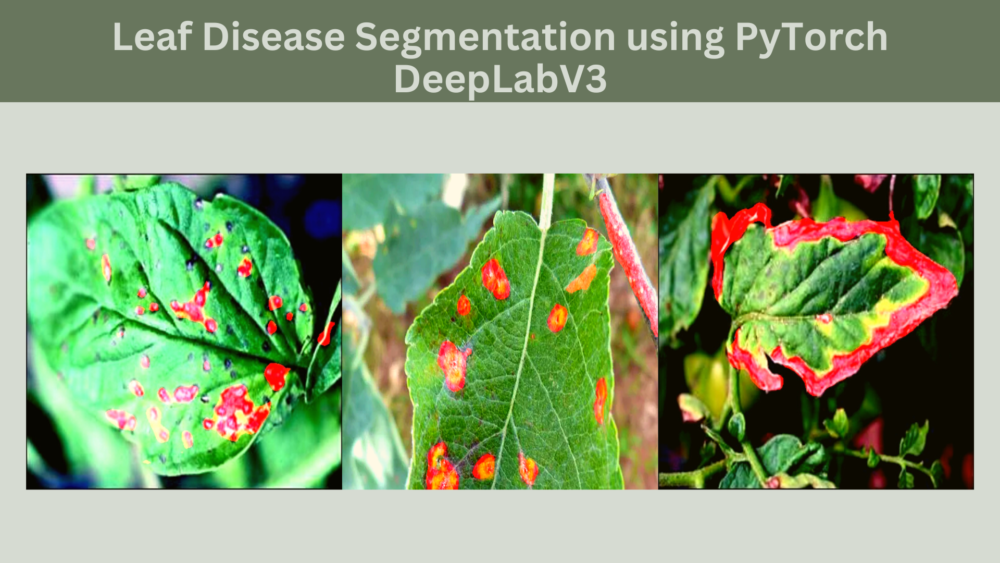
Disease detection using deep learning is a great way to speed up the process of plant pathology. In most cases, we go with either image classification or disease (object) detection when using deep learning. But we can use semantic segmentation as well. In some cases, leaf disease recognition with semantic segmentation is much more helpful. This is because the deep learning model can output the region affected by the disease. To know the entire process, in this article, we will cover PyTorch and DeepLab for leaf disease segmentation.

Segmenting a specific region on a leaf or plant can be extremely challenging. Particularly, when the diseased region is not so large. There can be several types of diseases that can affect the leaves of a plant. Some diseases cover a larger area and some a very small area. While doing the leaf disease segmentation project, we will also analyze all these difficulties that a model may face.

For now, let’s list out all the topics that we will cover here:

• We will start with a discussion of the dataset that we will use for leaf disease segmentation.
• Then we will discuss the directory structure of the project.
• Next, we will move on to discuss the important parts of the code. As this project contains a lot of code (9 Python files), we will only focus on the important parts.
• Then we will fine-tune a pretrained PyTorch DeepLabV3 semantic segmentation model on the leaf disease dataset.
• Finally, we carry out inference on images.

The Leaf Disease Segmentation Dataset

For this project/article, we will use a variation of the leaf disease segmentation dataset. This dataset contains images of diseased leaves in their original form and also in augmented form. But the dataset does not contain a training/validation split.

I have prepared another dataset, with a training and validation split. You can find the dataset with train/validation split here. This is the dataset that we will use in this project. This also contains both, the original images, and the images with augmentations in the aug_data directory.

But we will use the original images and add augmentations into the training pipeline. Around 15% of the images are reserved for validation and the rest for training. This brings about 90 validation images, and 498 training images.

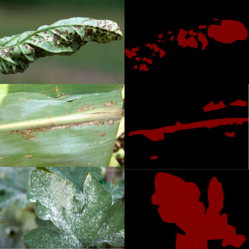
Here are a few images along with their masks from the training set.

After downloading the dataset, you should see the following directory structure.

├── aug_data
│   ├── train_images
│   ├── train_masks
│   ├── valid_images
│   └── valid_masks
└── orig_data
    ├── train_images
    ├── train_masks
    ├── valid_images
    └── valid_masks

We will use the images and masks from the orig_data directory.

Coming to the masks now. The masks in the leaves represent a disease that has affected it. Note that we do not segment different types of diseases. Instead, we just segment the areas of the leaves which is affected by a disease.

Also, in the ground truth mask, the diseased area on the leaf has a pixel value of (128, 0, 0) because of which it appears red. We need the pixel value information while preparing the dataset.

For now, please go ahead and download the leaf disease segmentation dataset with train/valid split.

The Project Directory Structure

Before moving on to the coding section, let’s take a look at the directory structure of the entire project.

.
├── input
│   └── leaf_disease_segmentation
│       ├── aug_data
│       └── orig_data
├── outputs
│   ├── valid_preds
│   │   ├── e0_b21.jpg
│   │   ...
│   │   └── e9_b21.jpg
│   ├── accuracy.png
│   ├── best_model_iou.pth
│   ├── best_model_loss.pth
│   ├── loss.png
│   ├── miou.png
│   └── model.pth
└── src
    ├── config.py
    ├── datasets.py
    ├── engine.py
    ├── inference_image.py
    ├── inference_video.py
    ├── metrics.py
    ├── model.py
    ├── train.py
    └── utils.py

8 directories, 71 files

• We already went over the leaf_disease_segmentation directory above. This contains the dataset and the entire directory will reside inside the input directory.
• The outputs directory will contain all the outputs from the training and validation experiments.
• The src directory contains the source code files. There are 9 Python files in total. We will execute all the commands in the terminal within the src directory.

All the code files will be available when you download the zip file that comes with this post. You just need to download the dataset from Kaggle in case you want to run the training yourself. If you just want to use the trained models for inference, please download the models from here. After extracting, put them in the outputs directory.

Leaf Disease Segmentation using PyTorch DeepLabV3

Let’s dive into the practical details of this project now. Although we will not be able to go into all the details of the code files, we will still check out the following:

• Configuration file containing some global values.
• The deep learning model that we are using for semantic segmentation of leaf diseases.
• The dataset preparation strategy along with the augmentations.
• IoU and accuracy metrics.
• A small discussion of the utility and helper scripts.
• And the arguments available for training.

Download Code

The Configuration File

We have a config.py file that contains some global configuration values. We can use these across different Python modules by importing them.

ALL_CLASSES = ['background', 'disease']

LABEL_COLORS_LIST = [
    (0, 0, 0), # Background.
    (128, 0, 0),
]

VIS_LABEL_MAP = [
    (0, 0, 0), # Background.
    (255, 0, 0),
]

The ALL_CLASSES list contains the names of the classes in the dataset. As this is a binary segmentation dataset, apart from the leaves’ disease class, we also have the background class.

Next, we have the LABEL_COLORS_LIST. This is a list containing the RGB values in tuple format. These are the exact values as in the ground truth segmentation masks. We need these values in the datasets.py file for the proper preparation of the dataset.

We also have the VIS_LABEL_MAP list containing colors for visualization. As you may observe, we are using pure red color for inference visualizations which gives a much better contrast against the green leaves.

The DeepLabV3 Models

We are going to use the DeepLabV3 ResNet50 as our primary model to train on the dataset. This means that we will analyze the training results using this and also run inference using this. It is pretty easy to prepare the model as PyTorch (Torchvision) already contains a pretrained model.

We can just need a simple function for this.

def prepare_model(num_classes=2):
    model = deeplabv3_resnet50(weights='DEFAULT')
    model.classifier[4] = nn.Conv2d(256, num_classes, 1)
    model.aux_classifier[4] = nn.Conv2d(256, num_classes, 1)
    return model

We do need to change the output channels to the number of classes in the dataset for the classifier and aux_classifier layers though.

The model.py file also contains the code for DeepLabV3 MobileNetV3 Large model. We will just analyze the performance from this model on the leaf segmentation dataset to compare with the ResNet50 one. But we will not run any inference experiments with this model. If you wish to train using this model, you may uncomment the lines in the model.py file.

The Dataset Preparation Strategy for Leaf Disease Segmentation

The most important part while preparing the dataset is the augmentation. From various experiments, I found that we need a myriad of augmentation to prevent the DeepLabV3 ResNet50 model from overfitting on this dataset.

Note: The overfitting was not that severe with the DeepLabV3 MobileNetV3 Large model even with less augmentation. But we need a lot of augmentation for the ResNet50 training.

Because of its easy usage, we are using the Albumentation library for augmentations in this project.

These are the final augmentations along with their probability values in brackets:

• HorizontalFlip (p=0.5)
• RandomBrightnessContrast (p=0.2)
• RandomSunFlare (p=0.2)
• RandomFog (p=0.2)
• Rotate (limit=50)
• ImageCompression (p=0.2)

These provide plenty of regularization. But as we will see later, we also need a few more things to regularize the training process even further.

In case you are wondering, here are some samples and how they look after random augmentations.

Only HorizontalFlip and Rotate are applied to both the image and ground truth mask. The rest are applied to the images only.

We do not apply augmentation to the validation dataset. But we normalize both the training and validation images according to the ImageNet normalization values. This is because we are using pretrained models and fine tuning them.

IoU and Accuracy Metrics

We will use IoU and accuracy metrics to evaluate the model. You can find the code for this in the metrics.py file which contains the IOUEval class.

I use the code for IoU and accuracy calculation from this repository as this contains some nice batch and history functionalities.

It is worthwhile to note something here. For saving the best model during training, we will use two criteria. We will save the model according to the least loss value for a current epoch and also when the model achieves the highest IoU.

Sometimes, the model with the least validation loss may not be the one with the highest IoU. Similarly, sometimes, the model with the highest IoU may be an overfit one according to the loss at that particular epoch.

Saving two different models will give us the choice to make an informed decision for choosing the best model for inference.

Utility and Helper Scripts

We will need several helper functions and classes while training the DeepLabV3 model for leaf disease segmentation.

The utils.py file contains all of these functions and classes. It is a pretty long file. So, here is a list of all the things it contains:

• set_class_values function to convert a specific integer to a particular class in the dataset.
• get_label_mask to encode the pixels belonging to the same class in the image into the same label.
• draw_translucent_seg_maps function to add the predicted segmentation map on one of the images during the validation loop and save it to disk. This helps to analyze the training process visually.
• SaveBestModel class to save the model according to the least loss.
• SaveBestModelIOU class to save the best model according to the highest IoU.
• save_model function to save the model one final time with the optimizer state dictionary. You may use this to resume training at a later point.
• save_plots function to save the loss, accuracy, and IoU graphs to disk.
• Transforms for inference.
• The get_segment_labels function to forward pass the image through the model during inference.
• draw_segmentation_map function to convert the predicted masks to RGB format.
• image_overlay function to overlay the RGB segmentation map on the image.

If you wish, you may go over utils.py file once before moving on to the training section.

Training the DeepLabV3 Model for Leaf Disease Segmentation

We will use the train.py script to start the training. Before jumping into the training experiments, let’s check out all the argument parsers that the training script supports.

• --epochs: The number of epochs we want to train the mode for.
• --lr: The learning rate for the optimizer. The default value is 0.0001.
• --batch: Batch size for the data loaders.
• --imgsz: The image resizing resolution while preparing the dataset. The default value is 512 which will resize the images to 512×512 resolution. We will use the default value only.
• --scheduler: This is a boolean argument indicating whether we want to apply any learning rate scheduling or not. If we pass this argument to the training script, then the learning rate will be reduced by a factor of 10 after every 20 epochs. This is a good way to check overfitting with larger models.

All the training and inference experiments were carried out on a system with 10 GB RTX 3080 GPU, 10th generation i7 CPU, and 32 GB of RAM.

DeepLabV3 ResNet50 Training

To start the training, we can execute the following command in the terminal by keeping src as the current working directory.

python train.py --epochs 50 --batch 4 --scheduler

We are using a batch size of 4 and an image resolution of 512×512. If you face an Out Of Memory (OOM) error, please reduce either the image size or batch size, or both and proceed further.

Here are some of the outputs from the terminal.

Namespace(epochs=50, lr=0.0001, batch=4, imgsz=512, scheduler=True)
41,994,308 total parameters.
41,994,308 training parameters.
Adjusting learning rate of group 0 to 1.0000e-04.
EPOCH: 1
Training
|                    | 125/? [01:29<00:00,  1.40it/s]                                                                                                                                         
Validating
|                    | 23/? [00:04<00:00,  5.15it/s]                                                                                                                                          

Best validation loss: 0.2707192062035851

Saving best model for epoch: 1


Best validation IoU: 0.6108606394368111

Saving best model for epoch: 1

Train Epoch Loss: 0.4412, Train Epoch PixAcc: 0.8103, Train Epoch mIOU: 0.536401
Valid Epoch Loss: 0.2707, Valid Epoch PixAcc: 0.8554 Valid Epoch mIOU: 0.610861
Adjusting learning rate of group 0 to 1.0000e-04.
--------------------------------------------------
.
.
.
EPOCH: 47
Training
|                    | 125/? [01:26<00:00,  1.45it/s]                                                                                                                                         
Validating
|                    | 23/? [00:04<00:00,  5.18it/s]                                                                                                                                          

Best validation loss: 0.1456461318809053

Saving best model for epoch: 47


Best validation IoU: 0.7550247198403427

Saving best model for epoch: 47

Train Epoch Loss: 0.1713, Train Epoch PixAcc: 0.9238, Train Epoch mIOU: 0.754309
Valid Epoch Loss: 0.1456, Valid Epoch PixAcc: 0.9028 Valid Epoch mIOU: 0.755025
Adjusting learning rate of group 0 to 1.0000e-06.
--------------------------------------------------
EPOCH: 48
Training
|                    | 125/? [01:26<00:00,  1.45it/s]                                                                                                                                         
Validating
|                    | 23/? [00:04<00:00,  5.16it/s]                                                                                                                                          

Best validation IoU: 0.7596472606104833

Saving best model for epoch: 48

Train Epoch Loss: 0.1744, Train Epoch PixAcc: 0.9207, Train Epoch mIOU: 0.746095
Valid Epoch Loss: 0.1499, Valid Epoch PixAcc: 0.9011 Valid Epoch mIOU: 0.759647
Adjusting learning rate of group 0 to 1.0000e-06.
--------------------------------------------------
EPOCH: 49
Training
|                    | 125/? [01:26<00:00,  1.44it/s]                                                                                                                                         
Validating
|                    | 23/? [00:04<00:00,  5.17it/s]                                                                                                                                          
Train Epoch Loss: 0.1708, Train Epoch PixAcc: 0.9229, Train Epoch mIOU: 0.752612
Valid Epoch Loss: 0.1483, Valid Epoch PixAcc: 0.9017 Valid Epoch mIOU: 0.753524
Adjusting learning rate of group 0 to 1.0000e-06.
--------------------------------------------------
EPOCH: 50
Training
|                    | 125/? [01:26<00:00,  1.44it/s]                                                                                                                                         
Validating
|                    | 23/? [00:04<00:00,  5.21it/s]                                                                                                                                          
Train Epoch Loss: 0.1848, Train Epoch PixAcc: 0.9169, Train Epoch mIOU: 0.736219
Valid Epoch Loss: 0.1501, Valid Epoch PixAcc: 0.9019 Valid Epoch mIOU: 0.754699
Adjusting learning rate of group 0 to 1.0000e-06.
--------------------------------------------------
TRAINING COMPLETE

We get the best IoU + best validation loss on epoch 47. But again on epoch 48, we get the best model as the IoU improved. This model was saved as best_model_iou.pth in the outputs directory. We will use this model for the inference experiments further.

Here are the loss, IoU, and accuracy plots after training.

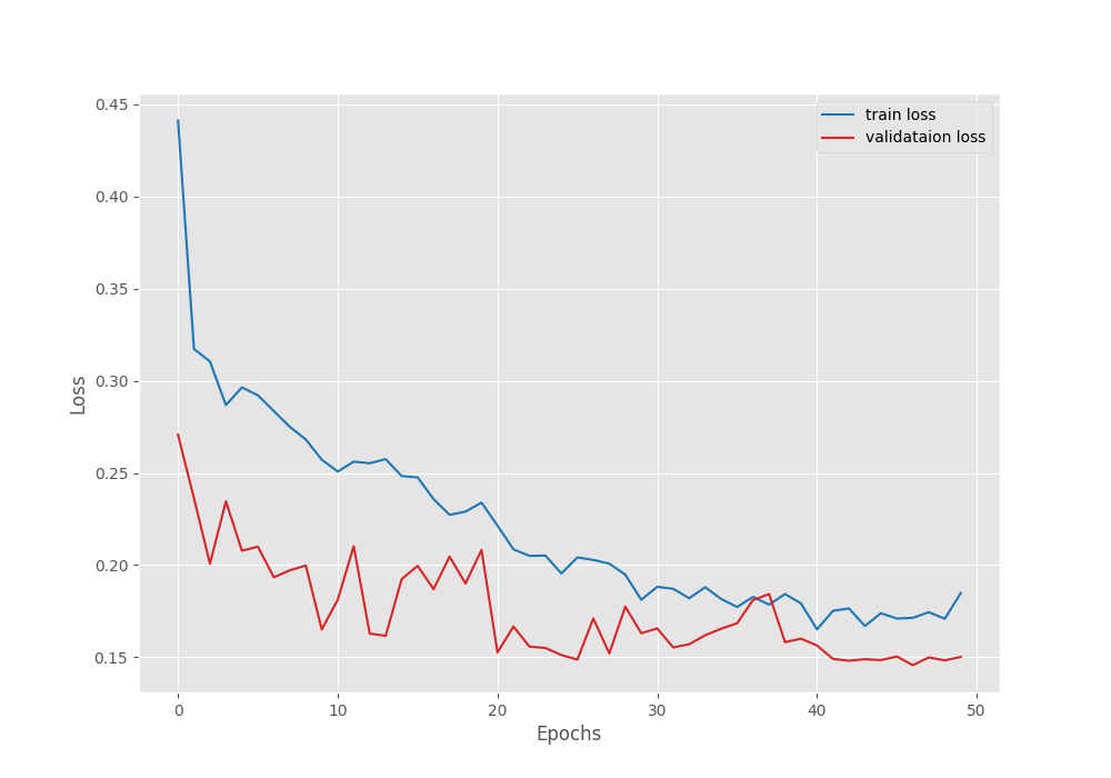
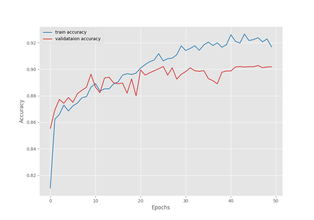
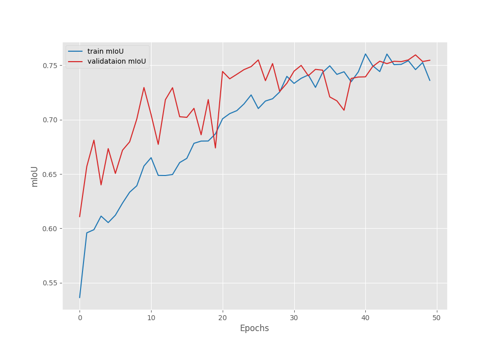
The learning rate schedule that we chose seems to be working pretty well. As we can see, the fluctuations in all three graphs seem to reduce after each of the learning rate schedule periods.

We have the best validation mIoU (mean IoU) of 75.5.

DeepLabV3 MobileNetV3 Large Results

In case you are curious, here are the results for DeepLabV3 MobileNetV3 Large training.

• Best validation loss: 0.156
• Highest validation mIoU: 66.4

As we can see, the best validation mean IoU is substantially lower compared to the ResNet50 results.

You have access to both the trained weights. You may download the models from this Kaggle link before moving to the inference section.

Inference for Leaf Disease Segmentation using the Trained DeepLabV3 Model

Let’s use the best DeepLabV3 ResNet50 weights and run some inference experiments.

Inference on Images

We will use the inference_images.py script to run inference on the validation images from the dataset. That way we can easily compare the results as we have the ground truth masks as well.

python inference_image.py --model ../outputs/best_model_iou.pth --input ../input/leaf_disease_segmentation/orig_data/valid_images/

In the above command, we provide the path to the best model using --model flag and the path to the data directory using the --input flag

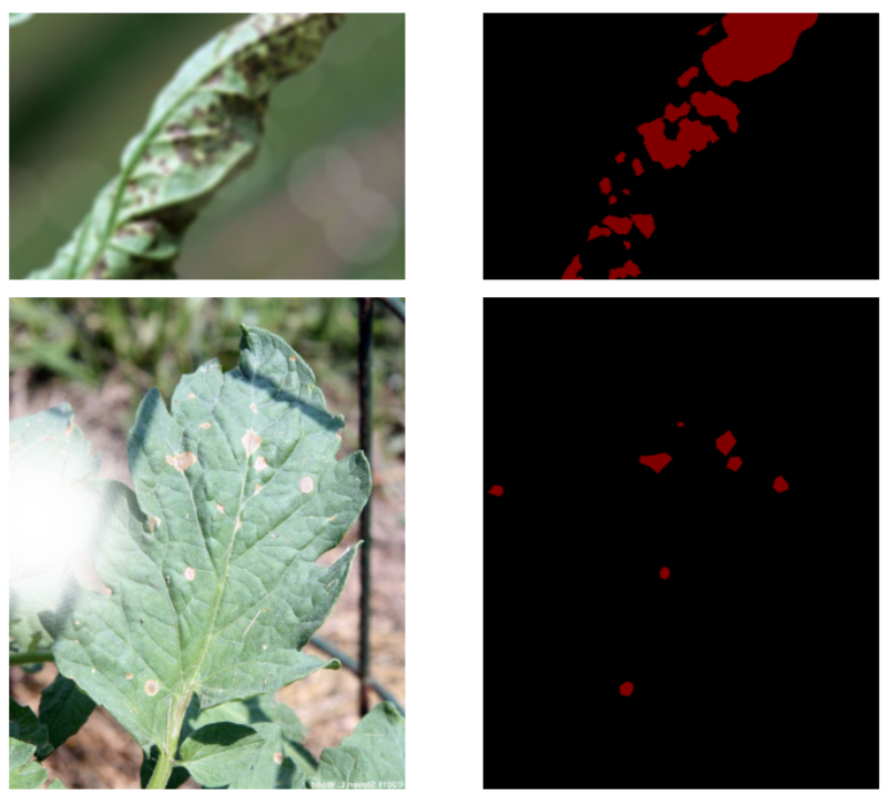
Here are some of the good segmentation results.

As you can see, the results may not be perfect, but they are pretty good. The model is able to segment even the small areas of diseases on the leaves.

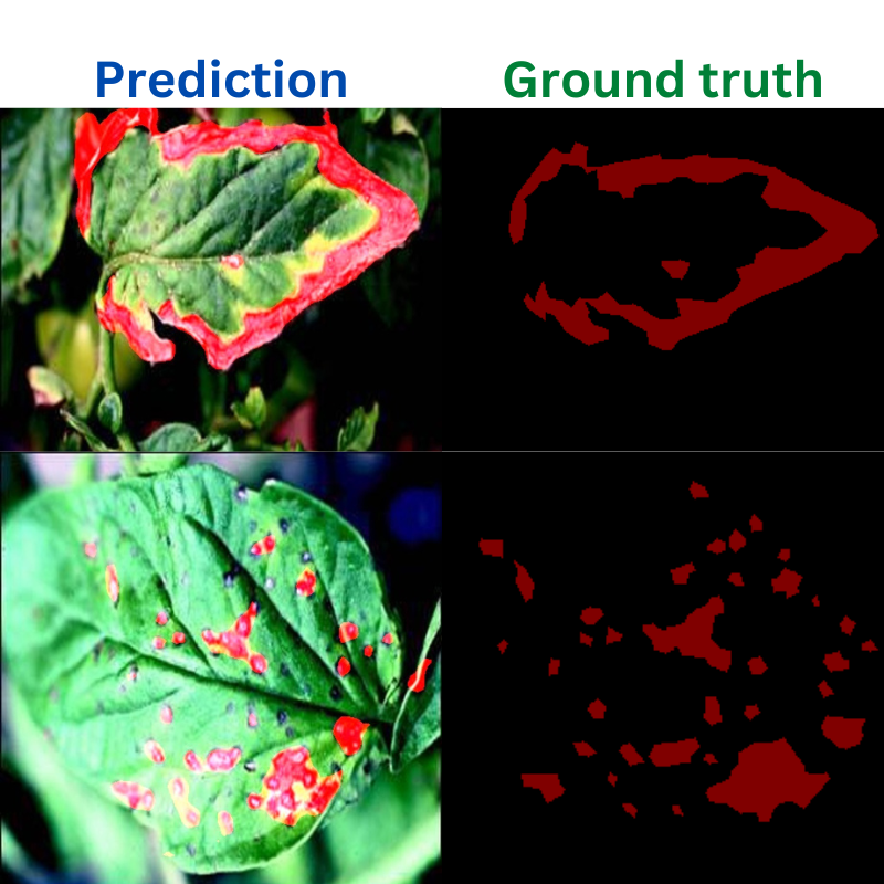
The following figure shows some results where the model failed to properly segment the diseased areas on the leaves.

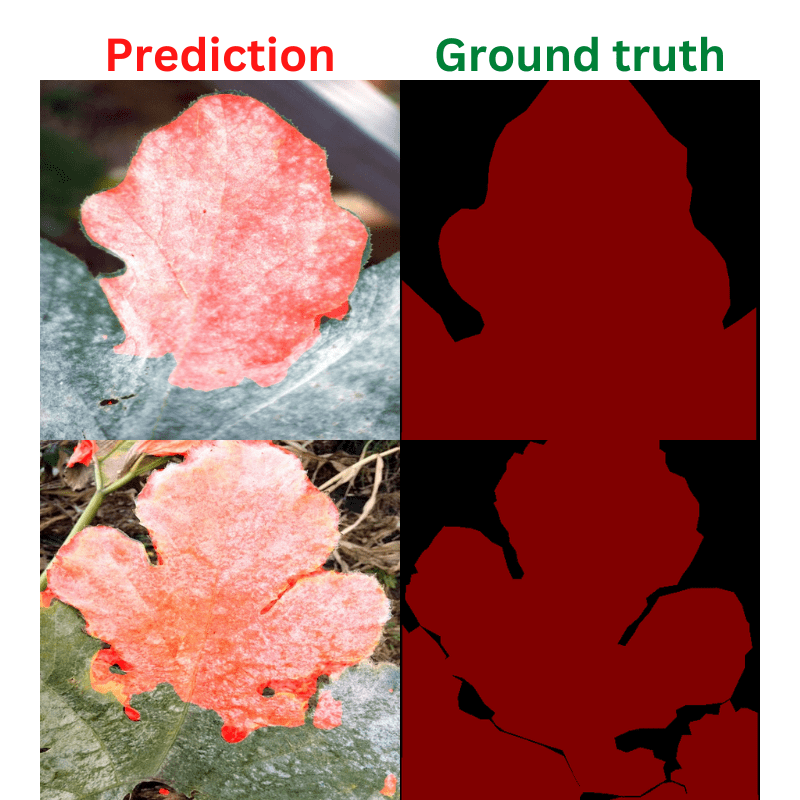
In the above examples, the model is unable to predict the entire region of the disease on the leaves.

Inference on Unseen Images

For the final experiment, let’s run inference on some unseen images from the internet. The data resides in the input/inference_data directory.

python inference_image.py --model ../outputs/best_model_iou.pth --input ../input/inference_data/images/

Following are some of the results.

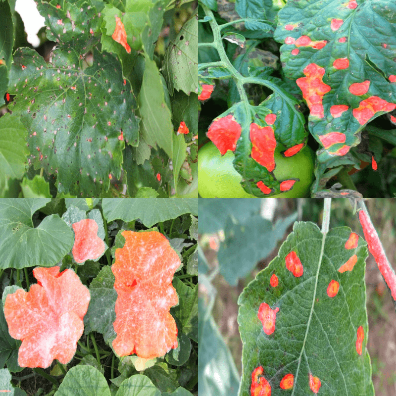
Although the ground truth data is not present, we can see that the results are very good. The model is even able to segment the very small diseased areas on the leaves.

Note: The src directory also contains an inference_video.py file. If you wish, you can run inference on videos right away by providing the model and video paths while executing the script.

Summary and Conclusion

In this article, we trained a DeepLabV3 model for semantic segmentation of leaf disease. After going through the entire process, we go to know how the model performs on validation images. To improve the performance even further, we can collect more such images for training. One other option is to train a larger model like DeepLabV3 with the ResNet101 backbone. But that also needs more GPU memory and is slower to train. If you carry out any more experiments, please share your findings in the comment section.

I hope that that article was worthy of your time.

If you have any doubts, thoughts, or suggestions, please leave them in the comment section. I will surely address them.

You can contact me using the Contact section. You can also find me on LinkedIn, and Twitter.