Semantic Segmentation using PyTorch DeepLabV3 and Lite R-ASPP with MobileNetV3 Backbone

Deep learning based semantic segmentation models often struggle to run in real-time. When applying semantic segmentation to videos, generally, the FPS (Frames Per Second) is not very good. But the scenario has been changing with some recent models and implementations. In this tutorial, we will apply semantic segmentation using PyTorch and try to get good FPS even on videos. Specifically, we will be applying semantic segmentation using PyTorch DeepLabV3 and Lite R-ASPP with MobileNetV3 backbone.

In the previous post we used the PyTorch DeepLabV3 semantic segmentation model with a ResNet50 backbone to apply semantic segmentation on images and videos.

• (Last week): Semantic Segmentation using PyTorch DeepLabV3 ResNet50.
• (This week): Semantic Segmentation using pre-trained PyTorch DeepLabV3 and Lite R-ASPP with MobileNetV3 backbone.

In this post also, we will be applying semantic segmentation to images and videos. But we will be using very computation friendly version, that is DeepLabV3 and Lite R-ASPP models with MobileNetV3 backbone. Hopefully, we will be able to get more than 3 FPS that we got in the last post with the ResNet50 backbone.

So, what are we going to cover in this tutorial?

• A brief about the DeepLabV3 and Lite R-ASPP models that we will be using.
  • What kind of input they expect and what outputs they give?
  • Also, what are the classes they have been trained on?
• The project directory structure and PyTorch version.
• Covering the coding part and applying semantic segmentation to images and videos using PyTorch DeepLabV3 and Lite R-ASPP models.

Let us get dive into the tutorial now.

The DeepLabV3 and Lite R-ASPP models with MobileNetV3 Backbone

We will not go over the models or architectures in very much detail here. They obviously require their own dedicated articles to do them proper justice.

As for the DeepLabV3 model, we went over some of the important concepts of it in the previous tutorial. They are the encoder-decoder architecture of the model, atrous convolution, and spatial pyramid pooling. Please go through the previous tutorial (Semantic Segmentation using PyTorch DeepLabV3 ResNet50) to know about these in a bit more detail.

Coming to the Lite R-ASPP (Lite Reduced Atrous Spatial Pyramid Pooling) model. According to the paper, Searching for MobileNetV3, it is a segmentation decoder architecture. This architecture is mostly suitable for mobile classification, detection, and segmentation. This means that it is fast and can run easily on mobile/edge/low-powered devices. Our main focus is the task of semantic segmentation here. And the LR-ASPP is a very lightweight head for semantic segmentation.

And by now, many of you must have noted that both the model, DeepLabV3 and Lite R-ASPP have a MobileNetV3 backbone which is very computationally feasible in itself.

So, all in all, we should be getting really good FPS in videos when using these models for semantic segmentation. One question that arises here, “will there be reduction in segmentation quality in exchange for faster runtime?”. Well, most probably, yes. And we will get to know the extent of that segmentation quality hit when we write the code and execute it.

As implied before, we will not go into any more details of the models’ architectures here. Rather, we will cover them in future articles.

The Dataset the Models Have Been Trained On

Both, the DeepLabV3 and the Lite R-ASPP model have been pre-trained on the MS COCO 2017 training dataset. But they have been trained only with the Pascal VOC classes.

The Pascal VOC has 21 classes including the __background__ class. The following are the classes on which both the PyTorch semantic segmentation models have been trained on.

['__background__', 'aeroplane', 'bicycle', 'bird', 'boat', 'bottle', 'bus',
 'car', 'cat', 'chair', 'cow', 'diningtable', 'dog', 'horse', 'motorbike',
 'person', 'pottedplant', 'sheep', 'sofa', 'train', 'tvmonitor']

This means that while carrying out inference, the DeepLabV3 and the Lite R-ASPP models will be able to segment 20 different objects in a single image/frame. This is going to be really interesting.

The Input and Output Format

All the PyTorch pre-trained semantic segmentation models expect the input in the same format. We will need to convert them into PyTorch image tensors. This will load the pixels in the range [0, 1]. This is what the models expect. We will also need to normalize the input image tensors using mean = [0.485, 0.456, 0.406] and std = [0.229, 0.224, 0.225]. These steps will become even clearer while coding.

Now, coming to the output format. Just like the input format, all the PyTorch pre-trained semantic segmentation models give the output in the same format. This makes switching between different models really easy. The models output an Ordered Dictionary in which the out key contains all the output tensors. For examples, the following is an output after feeding an input tensor and forward passing it through one of the PyTorch semantic segmentation models.

<class 'collections.OrderedDict'>
torch.Size([1, 21, 850, 1280])
OrderedDict([('out', tensor([[[[11.1675, 11.1675, 11.1675,  ...,  9.8225,  9.8225,  9.8225],
          [11.1675, 11.1675, 11.1675,  ...,  9.8225,  9.8225,  9.8225],
          [11.1675, 11.1675, 11.1675,  ...,  9.8225,  9.8225,  9.8225],
          ...,
          [ 6.0362,  6.0362,  6.0362,  ...,  9.5510,  9.5510,  9.5510],
          [ 6.0362,  6.0362,  6.0362,  ...,  9.5510,  9.5510,  9.5510],
          [ 6.0362,  6.0362,  6.0362,  ...,  9.5510,  9.5510,  9.5510]],
         [[ 0.5891,  0.5891,  0.5891,  ..., -2.3955, -2.3955, -2.3955],
          [ 0.5891,  0.5891,  0.5891,  ..., -2.3955, -2.3955, -2.3955],
          [ 0.5891,  0.5891,  0.5891,  ..., -2.3955, -2.3955, -2.3955],
          ...,
          [ 0.3087,  0.3087,  0.3087,  ...,  0.4327,  0.4327,  0.4327],
          [ 0.3087,  0.3087,  0.3087,  ...,  0.4327,  0.4327,  0.4327],
          [ 0.3087,  0.3087,  0.3087,  ...,  0.4327,  0.4327,  0.4327]],
         [[-0.8241, -0.8241, -0.8241,  ..., -1.9793, -1.9793, -1.9793],
          [-0.8241, -0.8241, -0.8241,  ..., -1.9793, -1.9793, -1.9793],
          [-0.8241, -0.8241, -0.8241,  ..., -1.9793, -1.9793, -1.9793],
          ...,
          [ 0.1900,  0.1900,  0.1900,  ..., -1.3187, -1.3187, -1.3187],
          [ 0.1900,  0.1900,  0.1900,  ..., -1.3187, -1.3187, -1.3187],
          [ 0.1900,  0.1900,  0.1900,  ..., -1.3187, -1.3187, -1.3187]],
         ...,

The above block contains a few extra pieces of information as well. For example, the shape of the output tensor. That is, [1, 21, 850, 1280]. This tells us that the model inferred on a batch containing a single image, has 21 output classes, and the output size is 1280×850 (width x height).

If you wish to know a bit more about the input and output formats, then please visit the Semantic Segmentation using PyTorch FCN ResNet post. There, we discuss these in a bit more detail with image illustrations.

Semantic Segmentation using PyTorch FCN ResNet

Directory Structure and PyTorch Version

As usual, we will follow a simple and efficient directory structure.

├── input
│   ├── image_1.jpg
│   ├── image_2.jpg
│   ├── video_1.mp4
│   └── video_2.mp4
├── outputs
│   ├── image_1.jpg
│   ├── image_2.jpg
│   ├── video_1.mp4
│   └── video_2.mp4
├── label_color_map.py
├── segmentation_utils.py
├── segment_image.py
└── segment_video.py

• First, we have an input folder in which there are 2 images and 2 videos that we will apply semantic segmentation to using the models. The two images and one of the videos are actually the same ones from the previous post. There we tested a DeepLabV3 model with ResNet50 backbone. Using a few similar images and videos will also let us compare the quality of segmentation and the FPS on videos. The second video is a new one.
• Second, the output folder will contain the output images and videos after they have passed through the model. They will have a semantic segmentation color map overlayed on them.
• Then we have four Python files. These are almost similar to the ones in the previous post. We will get to know more while going through each of them.

You can download the zip file for input test data and the source code by clicking on the button below. You are free to use any of your own images and videos as well.

The PyTorch Version

All the code in this tutorial uses PyTorch 1.8.0. You should be fine if you use either version 1.8.0 or any higher version that has been released at the time you are reading this.

Also, if you have an older PyTorch version, then it is a good idea to install the latest one. PyTorch gets many good updates with each iteration and you will be able to use them as well. Be sure to install them in a new Anaconda environment or Python virtual environment, whichever you use.

There are other dependencies such as OpenCV. But most probably, you already have them. Just install them on the go if you do not have any of the module/libraries required.

Semantic Segmentation using PyTorch DeepLabV3 and Lite R-ASPP

We will now dive into the coding part of this tutorial. We will write the code in all the four Python files that we discussed before.

Note: The detailed explanation of most of the code that we will cover in this post has already been covered in the last tutorial. So, we will go over the code explanations very lightly and dive deep only where new code is introduced.

Let us start with the coding part then.

Creating Label Color Map List for Each Segmentation Class

There are 21 classes in total including the background class. This means that, to visualize each of the segmented class properly, we will need to assign a different color map to them.

The label_color_map.py Python file contains a list called label_color_map. This list in-turn contains 21 tuples, each holding RGB (Red, Green, and Blue) color intensities for the 21 classes.

label_color_map = [
               (0, 0, 0),  # background
               (128, 0, 0), # aeroplane
               (0, 128, 0), # bicycle
               (128, 128, 0), # bird
               (0, 0, 128), # boat
               (128, 0, 128), # bottle
               (0, 128, 128), # bus 
               (128, 128, 128), # car
               (64, 0, 0), # cat
               (192, 0, 0), # chair
               (64, 128, 0), # cow
               (192, 128, 0), # dining table
               (64, 0, 128), # dog
               (192, 0, 128), # horse
               (64, 128, 128), # motorbike
               (192, 128, 128), # person
               (0, 64, 0), # potted plant
               (128, 64, 0), # sheep
               (0, 192, 0), # sofa
               (128, 192, 0), # train
               (0, 64, 128) # tv/monitor
]

That’s it for the label_color_map.py Python file. This just contains a list holding 21 tuples of RGB color values.

Image Segmentation Utility Code

We need to write some utility code and helper functions that will make the semantic segmentation part easier for us. Essentially, these helper functions will do the heavy lifting for us when invoked.

All these utility code will go into the segmentation_utils.py Python file.

The following are the import statements and modules that we will need along the way.

import torchvision.transforms as transforms
import cv2
import numpy as np
import torch

from label_color_map import label_color_map as label_map

Along with all the standard modules, we are also importing the label_color_map module that we wrote in the previous section.

The next block of code defines the image transforms that we will need to transform the input image pixels.

# define the torchvision image transforms
transform = transforms.Compose([
    transforms.ToTensor(),
    transforms.Normalize(mean=[0.485, 0.456, 0.406],
                         std=[0.229, 0.224, 0.225])
])

Next, we will define three functions that will help us in carrying our semantic segmentation, drawing the segmentation map, and overlaying the translucent segmentation map over the original RGB image.

Function to Obtain the Segmentation Labels

We will write a very simple function that will convert the image to tensor, forward pass it through the semantic segmentation model, and return the outputs.

def get_segment_labels(image, model, device):
    # transform the image to tensor and load into computation device
    image = transform(image).to(device)
    image = image.unsqueeze(0) # add a batch dimension
    outputs = model(image)
    return outputs

The get_segment_labels() function accepts three input parameters. They are the original image, the deep learning model, and the computation device.

Function to Draw the Segmentation Map

We need to get the segmentation maps according to the output that deep learning model provides us.

Each class in the segmentation map will have a different colored pixel and each object belonging to the same class will have the same colored pixel. The following code block achieves this.

def draw_segmentation_map(outputs):
    labels = torch.argmax(outputs.squeeze(), dim=0).detach().cpu().numpy()

    # create Numpy arrays containing zeros
    # later to be used to fill them with respective red, green, and blue pixels
    red_map = np.zeros_like(labels).astype(np.uint8)
    green_map = np.zeros_like(labels).astype(np.uint8)
    blue_map = np.zeros_like(labels).astype(np.uint8)
    
    for label_num in range(0, len(label_map)):
        index = labels == label_num
        red_map[index] = np.array(label_map)[label_num, 0]
        green_map[index] = np.array(label_map)[label_num, 1]
        blue_map[index] = np.array(label_map)[label_num, 2]
        
    segmentation_map = np.stack([red_map, green_map, blue_map], axis=2)
    return segmentation_map

The above function will return the segmentation_map where the background will be completely black and the objects will have colored coded pixels.

Function to Overlay the Segmentation Map on the Original Image

This is the final helper function that we will be writing. The image_overlay() function will overlay the segmentation map on the original RGB image. We will add a bit of translucency to the above segmentation map so that we can also see the objects beneath it and judge whether the deep learning model has correctly segmented the objects or not.

def image_overlay(image, segmented_image):
    alpha = 1 # transparency for the original image
    beta = 0.8 # transparency for the segmentation map
    gamma = 0 # scalar added to each sum

    segmented_image = cv2.cvtColor(segmented_image, cv2.COLOR_RGB2BGR)
    image = np.array(image)
    image = cv2.cvtColor(image, cv2.COLOR_RGB2BGR)
    cv2.addWeighted(image, alpha, segmented_image, beta, gamma, image)
    return image

The image that the above function returns is the final output that we need and will visualize after running the code.

We did not go through the code in detail in the above sections. Please go through the previous blog if you are interested in understanding the code in more depth.

Semantic Segmentation using PyTorch DeepLabV3 and Lite R-ASPP in Images

In this section, we will write the code to carry out inference and apply semantic segmentation to images. Then in the next section, we will move over to videos as well.

The semantic segmentation for images code will go into the segment_image.py Python script.

Let us start with importing all the modules that we will need for this script.

import torchvision
import torch
import argparse
import segmentation_utils
import cv2

from PIL import Image

• We need the torchvision module to load the DeepLabV3 and Lite R-ASPP models.
• The PIL Image module will help us in reading the images and cv2 module will help us in visualizing and saving the resulting segmented images.
• We are also importing our segmentation_utils module which contains the utility codes and helper functions.

Construct the Argument Parser and Define the Computation Device

We will be passing the image paths and the model names that we want to use as command line arguments. So, we will need an argument parser to parse those arguments.

# construct the argument parser
parser = argparse.ArgumentParser()
parser.add_argument('-i', '--input', help='path to input image')
parser.add_argument('-m', '--model', help='name of the model to use',
                    choices=['deeplabv3', 'lraspp'], required=True)
args = vars(parser.parse_args())

# set computation device
device = torch.device('cuda' if torch.cuda.is_available() else 'cpu')

We have two flags.

• One is the --input flag for the input image path.
• The other one is the --model flag. This will either accept deeplabv3 or lraspp as the model name according to which the respective model will be loaded by the torchvision module.

At line 16, we are also defining the computation device. It is always better to have a GPU for the purpose of semantic segmentation. Although for images, it is not mandatory, for videos, a GPU can provide a good FPS boost.

Load the Semantic Segmentation Model

We will load the appropriate semantic segmentation model according to the name provided for the --model flag in the command line arguments.

# load the model according to the --model flag
if args['model'] == 'deeplabv3':
    print('USING DEEPLABV3 WITH MOBILENETV3 BACKBONE')
    model = torchvision.models.segmentation.deeplabv3_mobilenet_v3_large(pretrained=True)
elif args['model'] == 'lraspp':
    print('USING LITE R-ASPP WITH MOBILENETV3 BACKBONE')
    model = torchvision.models.segmentation.lraspp_mobilenet_v3_large(pretrained=True)
# model to eval() model and load onto computation devicce
model.eval().to(device)

At lines 18 and 21, we are checking the name provided for the --model flag. If the name is deeplabv3, then we load the DeepLabV3 semantic segmentation model with MobileNetV3 Large backbone (line 20). Else if the model name provided is lraspp, then we load the Lite R-ASPP model with the MobileNetV3 Large backbone (line 23).

Note that in both cases, we are loading the trained weights which is really important. At line 25, we are switching the model into evaluation mode and loading it onto the computation device.

Reading the Image and Carrying Semantic Segmentation Inference

In the next code block we will:

• Read the image from the disk.
• Pass it through the model after pre-processing and obtain the segmentation label outputs.
• Draw the segmentation map on a black background.
• Over the segmentation map on the original image.
• Visualize the image on the screen and save the resulting segmented image to disk.

We are carrying all the above steps in the following code block.

# read the image
image = Image.open(args['input'])
# do forward pass and get the output dictionary
outputs = segmentation_utils.get_segment_labels(image, model, device)
# get the data from the `out` key
outputs = outputs['out']
segmented_image = segmentation_utils.draw_segmentation_map(outputs)

final_image = segmentation_utils.image_overlay(image, segmented_image)
save_name = f"{args['input'].split('/')[-1].split('.')[0]}_{args['model']}"
# show the segmented image and save to disk
cv2.imshow('Segmented image', final_image)
cv2.waitKey(0)
cv2.imwrite(f"outputs/{save_name}.jpg", final_image)

This completes the code for semantic segmentation on images. Let us now execute the code and analyze the results.

Execute segment_image.py Script to Apply Semantic Segmentation to Images

We have two images in the input folder. We will run both the images through both the models and analyze the quality of segmentation.

Using DeepLabV3 with MobileNetV3 Backbone

First, we will pass both the images through the DeepLabV3 model. Head over to the project directory, open up your terminal and type the following command.

python segment_image.py --input input/image_1.jpg --model deeplabv3

You will see a short message on the terminal stating the model name which is being loaded. Let us check that out just once.

USING DEEPLABV3 WITH MOBILENETV3 BACKBONE

In this case, we are loading the DeepLabV3 model as the --model flag is deeplabv3.

The following is the output that we get.

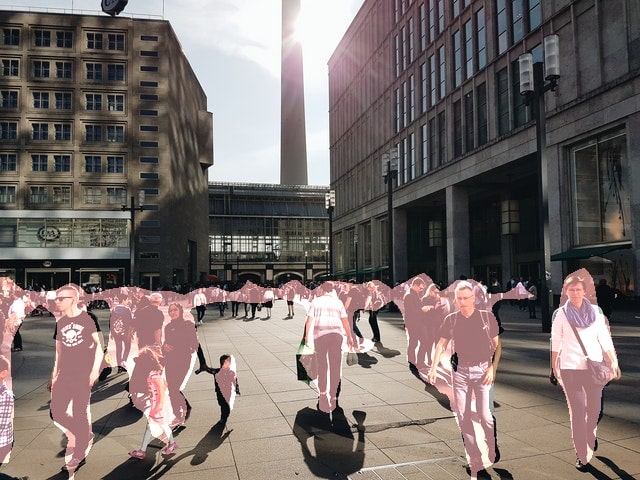
The segmentation maps are good for the persons who are closer to the camera and appear bigger. But the model is not able to segment the persons at the back properly. Even the small child at the front does not have very good segmentation map.

Now, if we compare it to the previous post where we used DeepLabV3 with ResNet50 backbone, then those results were really good. The people at the front had much better segmentation maps when compared to the MobileNetV3 backbone. This is the trade-off we need to consider when switching to a lighter backbone encoder like MobileNetV3.

Let us try with the second image. This image is a really challenging one.

python segment_image.py --input input/image_2.jpg --model deeplabv3

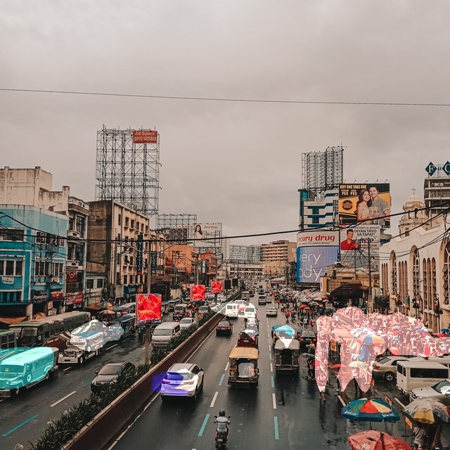
This time the results are even worse. The model is hardly able to segment any objects properly in the image. We can only see some blue patches for the car, and greenish-blue patches for the bus. All the persons are segmented as one whole object. In case of the DeepLabV3 with ResNet50 backbone, the segmentation maps for the vehicles were much better.

Using Lite R-ASPP with MobileNetV3 Backbone

Let us keep in mind the LR-ASPP model is even more lightweight than the DeepLabV3 model. And then it is paired with a MobileNetV3 backbone. So, it is going to be really challenging for the model.

Starting with the first image.

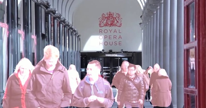
python segment_image.py --input input/image_1.jpg --model lraspp

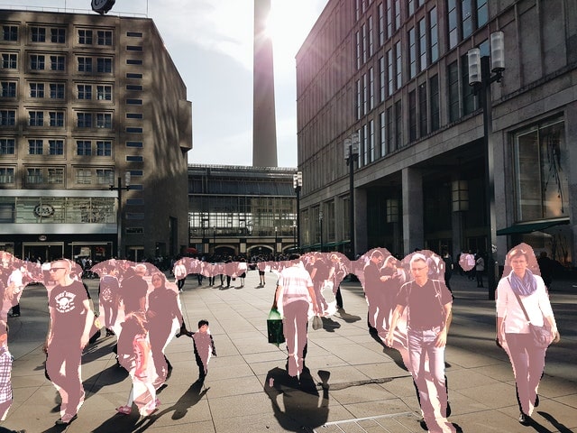
For the person segmentation, the results are not that bad. The segmentation maps are slightly worse than the DeepLabV3 case but still good.

Trying with the second image.

python segment_image.py --input input/image_2.jpg --model lraspp

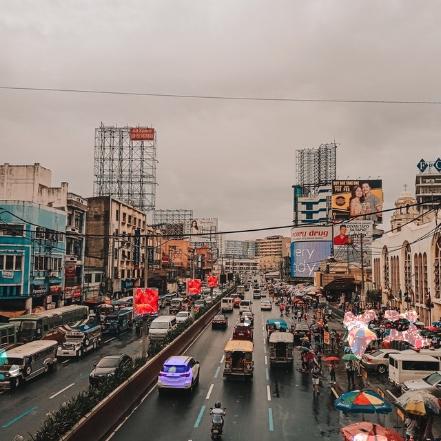
The LR-ASPP model with the MobileNetV3 backbone is not able to segment even a single vehicle. And the person segmentation at the right is also not acceptable.

But one thing to note here is that both, DeepLabV3 and Lite R-ASPP with the MobileNetV3 backbones are meant to be fast and give good FPS in videos. So, maybe they will able to make up for the segmentation speed in videos which they lacked in the quality of segmentation when given some difficult images to segment.

We will check that out in the next section.

Semantic Segmentation using PyTorch DeepLabV3 and Lite R-ASPP in Videos

It is time that we dive into semantic segmentation in videos now.

The code that we will write in this section will go into the segment_video.py Python script.

The code till the loading of the models will remain almost completely the same as was in the case of images. So, let us write that part first.

import torchvision
import cv2
import torch
import argparse
import time
import segmentation_utils

# construct the argument parser
parser = argparse.ArgumentParser()
parser.add_argument('-i', '--input', help='path to input video')
parser.add_argument('-m', '--model', help='name of the model to use',
                    choices=['deeplabv3', 'lraspp'], required=True)
args = vars(parser.parse_args())

# set the computation device
device = torch.device('cuda' if torch.cuda.is_available() else 'cpu')

# download or load the model from disk
if args['model'] == 'deeplabv3':
    print('USING DEEPLABV3 WITH MOBILENETV3 BACKBONE')
    model = torchvision.models.segmentation.deeplabv3_mobilenet_v3_large(pretrained=True)
elif args['model'] == 'lraspp':
    print('USING LITE R-ASPP WITH MOBILENETV3 BACKBONE')
    model = torchvision.models.segmentation.lraspp_mobilenet_v3_large(pretrained=True)
# load the model onto the computation device
model = model.eval().to(device)

The only difference is that we will pass path to a video file instead of an image file to the --input flag.

Reading the Video File and Preliminary Setup

We will read the video file from the disk using OpenCV’s VideoCapture() object. Along with that, we will also create a VideoWriter() object and provide an appropriate name for the resulting frames to be saved to the disk.

cap = cv2.VideoCapture(args['input'])
if (cap.isOpened() == False):
    print('Error while trying to read video. Please check path again')

# get the frame width and height
frame_width = int(cap.get(3))
frame_height = int(cap.get(4))

save_name = f"{args['input'].split('/')[-1].split('.')[0]}_{args['model']}"
# define codec and create VideoWriter object
out = cv2.VideoWriter(f"outputs/{save_name}.mp4",
                      cv2.VideoWriter_fourcc(*'mp4v'), 30,
                      (frame_width, frame_height))

frame_count = 0 # to count total frames
total_fps = 0 # to get the final frames per second

The saved video name will contain deeplabv3 or lraspp at the end according to the model we choose while executing the script.

Additionally, we also have a frame_count and a total_fps variable to keep track of the total number of frames and total Frames Per Second at the end of the video.

Looping Over the Video Frames and Applying Semantic Segmentation to Each Frame

Next, we will loop through each frame of the video using a while loop and apply all the semantic segmentation steps to each frame just as we did in the case of images. In short, we will treat each frame as a single image.

The following code block contains the complete while loop.

# read until end of video
while(cap.isOpened()):
    # capture each frame of the video
    ret, frame = cap.read()
    if ret:
        rgb_frame = cv2.cvtColor(frame, cv2.COLOR_BGR2RGB)
        # get the start time
        start_time = time.time()
        with torch.no_grad():
            # get predictions for the current frame
            outputs = segmentation_utils.get_segment_labels(rgb_frame, model, device)
        
        # obtain the segmentation map
        segmented_image = segmentation_utils.draw_segmentation_map(outputs['out'])
        # get the final image with segmentation map overlayed on original iimage
        final_image = segmentation_utils.image_overlay(rgb_frame, segmented_image)

        # get the end time
        end_time = time.time()
        # get the current fps
        fps = 1 / (end_time - start_time)
        # add current fps to total fps
        total_fps += fps
        # increment frame count
        frame_count += 1
        # put the FPS text on the current frame
        cv2.putText(final_image, f"{fps:.3f} FPS", (20, 35),
                    cv2.FONT_HERSHEY_SIMPLEX, 1, (0, 255, 0), 2)
        # press `q` to exit
        cv2.imshow('image', final_image)
        out.write(final_image)
        if cv2.waitKey(1) & 0xFF == ord('q'):
            break
    else:
        break

We are looping over the video frames until there are no frames present in the file.

Starting from line 51, we are applying the operations to each video frame that we applied to the images in the previous section.

• First, we are obtaining the segmentation labels at line 53 by executing the get_segment_labels() function.
• Second, we are obtaining the segmentation map at line 56.
• And finally, we are overlaying the segmentation map on the original image by executing the image_overlay() function at line 58.

After that, the following code lines carry out the calculation of Frames Per Second, incrementing the frame counter, and putting the FPS text on the current frame. Finally, we visualize the video and save the resulting frames to the disk.

The final thing to do is closing all VideoCapture() objects, releasing the OpenCV windows, and printing the average FPS on the terminal.

# release VideoCapture()
cap.release()
# close all frames and video windows
cv2.destroyAllWindows()
# calculate and print the average FPS
avg_fps = total_fps / frame_count
print(f"Average FPS: {avg_fps:.3f}") 

This completes our code for semantic segmentation using PyTorch in videos as well.

Execute segment_video.py Script to Apply Semantic Segmentation to Videos

Now, we will execute segment_video.py script and analyze the video outputs of DeepLabV3 and Lite R-ASPP models. We will be running the models on two videos. One is the same as the previous blog post where we used the DeepLabV3 model with ResNet50 backbone. This will help us compare the FPS boost that we are getting with a lighter MobileNetV3 backbone and also the Lite R-ASPP model. The second video is a new one just to test the models.

Using DeepLabV3 with MobileNetV3 Backbone

We will start with the DeepLabV3 model and pass the video_1.mp4 file from the input directory.

python segment_video.py --input input/video_1.mp4 --model deeplabv3

On a GTX 1060 GPU, the average FPS was 20.221. Yours might lower or higher depending upon the GPU. The model will also run on a CPU quite fine. The FPS will be somewhere around 3-4 on a CPU. Now in the previous post with DeepLabV3 and ResNet50 backbone, we were getting somewhere around 3 FPS on a GTX 1060. Comparing that to 20 FPS, we have surely gained a lot of speed.

But what about the trade-off in segmentation quality?

The following is the output video that is saved to disk.

Frankly, the DeepLabV3 with MobileNetV3 backbone is not performing that badly. Obviously, the segmentation maps for the trees and bikes were better with the ResNet50 backbone. And the far away persons are segmented as one large blob here. Still, most of the segmentation maps are quite good.

Let us throw a bit easier video towards the model now, which contains only humans.

python segment_video.py --input input/video_2.mp4 --model deeplabv3

On an average, this was again around 20 FPS.

There is nothing much to judge here. Pre-trained semantic segmentation models are pretty good at labeling persons. And this is the case here too. For sure, any model with a larger backbone (like ResNet50) will give even better segmentation maps.

Using Lite R-ASPP with MobileNetV3 Backbone

Now, we will carry out semantic segmentation inference using the Lite R-ASPP model.

Starting with the first video.

python segment_video.py --input input/video_1.mp4 --model lraspp

The average FPS was 28.933, almost 29 FPS which is quite a big jump when compares with the DeepLabV3’s 20 FPS.

And as expected, the segmentation maps are worse when compared with DeepLabV3 MobileNetV3 backbone. It is not able to label almost any plant at all. And the segmentation maps for the bikes are not that good as well. Even the segmentation maps for the persons are somewhat off.

This is the trade-off we need to consider when aiming for speed. We will lose a lot of quality in terms of the segmentation labels and maps.

Now, a final test on the second video.

python segment_video.py --input input/video_2.mp4 --model lraspp

Here also, we are getting around 29 FPS on an average.

For such a video where persons are so close to the camera, the segmentation maps are okay at best. We were getting better segmentation maps with the DeepLabV3 MobileNetV3 backbone. At least, the speed makes up for the lack in segmentation quality.

Some Observations

• We carried out semantic segmentation inference using DeepLabV3 and Lite R-ASPP with MobileNetV3 backbone.
• The DeepLabV3 MobileNetV3 model was faster than the one with ResNet50 backbone. But the segmentation quality was not as good.
• The Lite R-ASPP model was the fastest, giving 29 FPS average on a video. But then again, the segmentation quality was also the worst.
• This shows that it is really difficult to obtain good segmentation maps and have great FPS on videos at the same time. Obviously, this gap will keep on reducing for semantic segmentation models in the coming years.

Summary and Conclusion

In this tutorial, we carried out semantic segmentation inference using DeepLabV3 and Lite R-ASPP PyTorch models, both with MobileNetV3 backbone. We got to know the trade-off we have to make in terms of segmentation quality when aiming for higher FPS in videos. I hope that you learned something new in this tutorial.

If you have any doubts, thoughts, or suggestions, then please leave them in the comment section. I will surely address them.

You can contact me using the Contact section. You can also find me on LinkedIn, and Twitter.