In this article, we will make additional improvements to our previous custom robust keypoint detection model. In addition to a faster face detection model, we will optimize the face keypoint regressor model, as well as the inference pipeline. All in all, this article is all about improving the face keypoint detection model and pipeline.
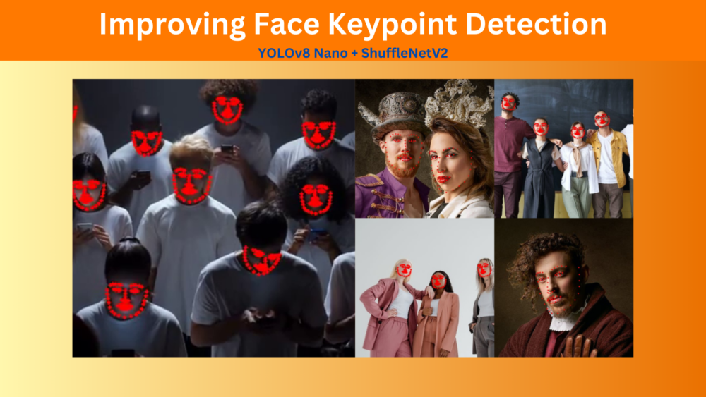
Figure 1. Improved face keypoint detection pipeline output.
We will cover the following topics in this article
We will start with a discussion of the issues with our previous approach to face keypoint detection.
Then we will move to the discussion of the changes that we will make to make the face keypoint detection pipeline faster.
Next, we will cover the code changes that we are making for improving the face keypoint detection. Overall, we aim to make the face keypoint detection pipeline around 2x faster while keeping the accuracy intact.
We will cover only the essential changes to the Python code files. You may go through the previous article to cover the code explanation in detail.
Issues with Previous Keypoint Detection Approach and Steps to Improving It
In our previous article, we used the pretrained MTCNN model for face detection and a custom ResNet50 model for facial keypoint detection. Primarily, there were two issues with the approach.
The pretrained MTCNN model was too slow.
The MTCNN model predicted too many false positives leading to false positives in face keypoint detection as well.
There are better and faster custom face detection models that will speed up the entire pipeline considerably.
In this article, we will specifically focus on the speed improvements. This needs a change in two components.
We will use a YOLOv8 model which has been custom trained on the WIDER Face dataset.
Along with that, we will train a smaller and faster face keypoint detection model. We will switch the model from ResNet50 to ShuffleNet.
Getting the Dataset
We will use the preprocessed dataset that we discussed in the first article. You can find the cropped dataset here on Kaggle.
You may also go through the previous article to learn more about the dataset preparation steps.
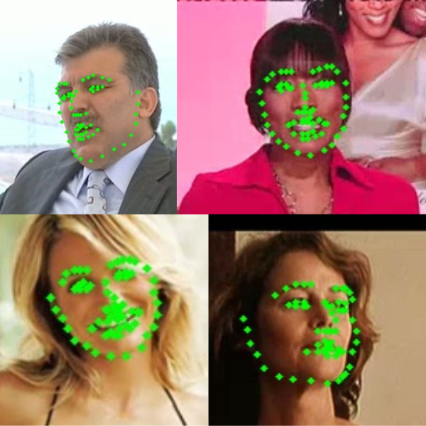
Figure 2. Facial keypoint detection ground truth dataset.
For brevity, here, we will only talk about the major changes and additions that we make to the dataset preparation steps.
Project Directory Structure
Let’s take a look at the directory structure before covering the code for improving the face keypoint detection.
Along with that, we also need the PyTorch framework. You can install it according to your configuration from the official website.
Improving Face Keypoint Detection
Let’s jump into the technical aspects and go through the code changes that we have to make for improving the speed and accuracy of our face keypoint detection pipeline.
In the previous article’s dataset preparation process, we did not apply any augmentations to the images. This time, we will apply augmentations to make the learning process of the model more robust. As we need to deal with keypoints as well, we will use the Albumentations library for augmentations.
Here are the additional training and validation augmentation & transforms that we define in the datasets.py file.
We apply random brightness & contrast, rotation, and random gamma augmentations to the training samples. We resize the samples to 224×224 resolution and apply the ImageNet normalization values as we will fine-tune a pretrained ShuffleNet model for the keypoint regression.
Additionally, we need to handle the keypoints as well. When we rotate an image horizontally, the keypoints need to be transformed accordingly. For this, we use the keypoint_params argument of Albumentations. We provide the keypoint format first. Ours will be the X and Y coordinates in a list for each image and therefore, we provide format='xy'. Furthermore, sometimes, during dataset preparation or augmentation, some keypoints may fall outside the image borders. To avoid value errors in Albumentations, we can pass remove_invisible=False.
Minor changes also happen in the FaceKeypointDataset class as we need not handle the resize and normalization manually.
The above are all the changes that we need for the dataset preparation step.
The ShuffleNet Model for Improving Keypoint Detection Speed
Previously, we used the ResNet50 model for the keypoint regression training and detection. However, it contains more than 25 million parameters. With proper augmentations and hyperparameters, we can train a much smaller model. This time, we will train one of the smallest ShuffleNetV2 models from PyTorch.
This is the entire dataset class that goes into the model.py file.
class FaceKeypointModel(nn.Module):
    def __init__(self, pretrained=False, requires_grad=True):
        super(FaceKeypointModel, self).__init__()
        if pretrained:
            self.model = shufflenet_v2_x0_5(weights='DEFAULT')
        else:
            self.model = shufflenet_v2_x0_5(weights=None)

        if requires_grad:
            for param in self.model.parameters():
                param.requires_grad = True
            print('Training intermediate layer parameters...')
        else:
            for param in self.model.parameters():
                param.requires_grad = False
            print('Freezing intermediate layer parameters...')

        # change the final layer
        self.model.fc = nn.Linear(in_features=1024, out_features=136)

    def forward(self, x):
        out = self.model(x)
        return out
The final model for our use contains just 481,192 parameters. We can use a much higher learning rate and a higher batch size.
Training the ShuffleNetV2 Model for Improving Face Keypoint Detection
Following are the hyperparameters for this training phase:
A batch size of 64
A learning rate of 0.001
And training for 100 epochs
You can find the details in the config.py file.
All the training and inference experiments were carried out on a system with 10 GB RTX 3080 GPU, 10th generation i7 CPU, and 32 GB RAM.
We can execute the following command to start the training.
python train.py
The training script saves the best model to disk whenever the validation loss reaches a new lower value. So, we get the best model in the end. Following are the logs from the best epoch.
Epoch 98 of 100
Training
100%|████████████████████| 54/54 [00:06<00:00, 7.89it/s]
Validating
0%| | 0/12 [00:00
The best model was obtained on epoch 98 with a validation loss of 3.2896.
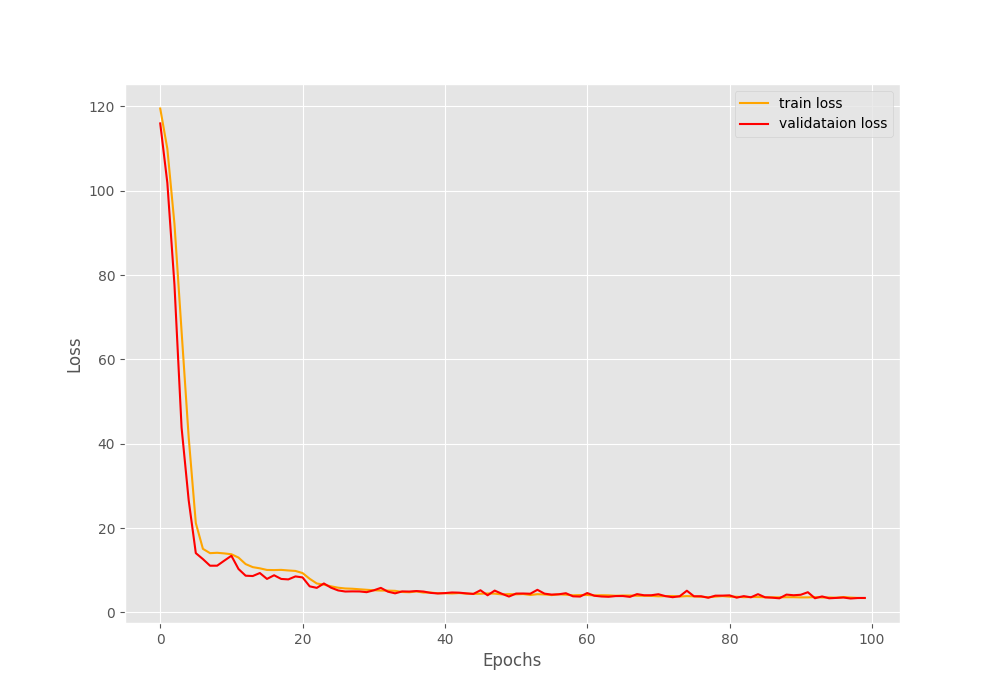
Here is the loss graph after training.
Figure 3. The loss graph while improving the face keypoint detection pipeline. It looks like with a bit of learning rate scheduling, we can train the model for even longer.
The YOLO Object Detection Model
We are using a YOLOv8 model which has been pretrained on the WIDER Face dataset for face detection. You can find the repository here. We are using the YOLOv8 Nano model from this repository and have kept it in the weights directory.
To optimize the inference process even further, we have exported the model to ONNX format using the export.py script to run on 320×320 resolution images.
Thanks to the Ultralytics library, the code for exporting it is pretty straightforward.
"""
Script to export YOLO face detection model.
"""
from ultralytics import YOLO
model = YOLO('weights/yolov8n_100e.pt')
model.export(format='onnx', imgsz=320)
You will get access to the original .pt file and also the ONNX format when downloading the zip file for this article.
Inference on Images
Let’s check the code to run inference on images. In this section, we will combine the detection outputs from the YOLOv8 model and our own keypoint detection model. A lot of the code will also remain similar to the previous post in the series. For a detailed explanation, I would recommend going through that post. The code for this resides in the inference_image.py script.
First, we have all the import statements.
import torch
import numpy as np
import cv2
import glob
import os
import albumentations as A
from model import FaceKeypointModel
from ultralytics import YOLO
from tqdm import tqdm
Next, we have the helper function to crop and pad the detected image.
Then we need to define the computation device, load both models, and define all the image paths.
device = torch.device('cuda:0' if torch.cuda.is_available() else 'cpu')
out_dir = os.path.join('outputs', 'image_inference')
os.makedirs(out_dir, exist_ok=True)
model = FaceKeypointModel(pretrained=False, requires_grad=False).to(device)
# Load the keypoint model checkpiont.
checkpoint = torch.load('outputs/model.pth')
model.load_state_dict(checkpoint['model_state_dict'])
model.eval()
# Load the YOLO model.
yolo = YOLO('weights/yolov8n_100e.onnx')
input_path = 'input/inference_images'
all_image_paths = glob.glob(os.path.join(input_path, '*'))
Finally, loop over the image paths and carry out the inference.
for image_path in tqdm(all_image_paths, total=len(all_image_paths)):
image_name = image_path.split(os.path.sep)[-1]
orig_image = cv2.imread(image_path)
with torch.no_grad():
results = yolo(orig_image, imgsz=320)
# Iterate over the YOLO `results` object.
for r in results:
# Detect keypoints if face is detected.
if len(r.boxes.xyxy) > 0:
for box in r.boxes.xyxy:
cropped_image, x1, y1 = crop_image(box, orig_image)
image = cropped_image.copy()
if image.shape[0] > 1 and image.shape[1] > 1:
image = cv2.resize(image, (224, 224))
image = image / 255.0
image = np.transpose(image, (2, 0, 1))
image = torch.tensor(image, dtype=torch.float)
image = image.unsqueeze(0).to(device)
with torch.no_grad():
outputs = model(image)
outputs = outputs.cpu().detach().numpy()
outputs = outputs.reshape(-1, 2)
keypoints = outputs
# Draw keypoints on face.
for i, p in enumerate(keypoints):
p[0] = p[0] / 224 * cropped_image.shape[1]
p[1] = p[1] / 224 * cropped_image.shape[0]
p[0] += x1
p[1] += y1
cv2.circle(
orig_image,
(int(p[0]), int(p[1])),
2,
(0, 0, 255),
-1,
cv2.LINE_AA
)
cv2.imwrite(os.path.join(out_dir, image_name), orig_image)
On lines 50 and 51, we pass the image through the YOLOv8 model to detect the faces. Then, for each result object, we only move forward with the keypoint detection if any faces are detected. If the YOLOv8 model detects faces, then we crop the face area along with padding on each side. Next, we pass this cropped face through the improved keypoint detection model. After each inference step, we annotate the image with the keypoints and save it to disk.
Let’s execute the script and check the results.
python inference_image.py
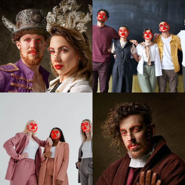
Figure 4. Image inference outputs after improving the face keypoint detection pipeline.
The results look good. However, we can see that if the faces are slightly tilted, then the keypoints are also a bit out of place. This can be easily solved with more data and variations in the training set.
Inference on Videos
Our main aim here is to improve the speed and accuracy that we had over our previous method. Let’s run inference on one of the same videos and check whether we succeed or not.
We run inference on videos by executing the inference_video.py script.
Clip 1. Real-time face keypoint detection using our improved pipeline. With the same video and using YOLOV8 ONNX model and a light weight keypoint regressor, we are able to reach more than 40 FPS compared to our previous method.
There are two major improvements that we can see right away:
There are way less false positives this time.
A boost in FPS leads to an average of 50 FPS on the same hardware.
However, whenever there are too many faces in a frame, the FPS still takes a hit.
Let’s try a video where there are multiple faces in almost all the frames.
Clip 2. The detection looks quite good here. However, when there are many faces in a single frame, the FPS takes a hit.
This time the FPS dips to an average of 7 FPS. This shows that our pipeline is not completely optimized as of yet.
Takeaways
We tried to improve our two-stage face keypoint detection as much as we could. There are a few more ways like converting the keypoint detection model to ONNX format as well but that will not help much with the speed. Although a bit slower with multiple faces, our face keypoint regression model can carry out detections from several angles and in different lighting conditions.
This shows that integrated single stage models may be faster but with a two stage pipeline, our detections are far superior. We can tune the face detection and keypoint detection models independently on hundreds of thousands of images.
In this article, we tried improving our two-stage keypoint detection pipeline in terms of speed. Along with a lightweight face detection model and converting it to ONNX, we also trained a much smaller keypoint regressor model. Although we were able to succeed to an extent, we also found potential drawbacks. We also discussed why single stage models may suit better for such use cases. I hope that this article was worth your time.
If you have any doubts, thoughts, or suggestions, please leave them in the comment section. I will surely address them.
You can contact me using the Contact section. You can also find me on LinkedIn, and X.
Liked it? Take a second to support Sovit Ranjan Rath on Patreon!
This website uses cookies so that we can provide you with the best user experience possible. Cookie information is stored in your browser and performs functions such as recognising you when you return to our website and helping our team to understand which sections of the website you find most interesting and useful.
Strictly Necessary Cookies
Strictly Necessary Cookie should be enabled at all times so that we can save your preferences for cookie settings.
If you disable this cookie, we will not be able to save your preferences. This means that every time you visit this website you will need to enable or disable cookies again.