Transfer Learning using PyTorch ShuffleNetV2

In this tutorial, we will carry out Transfer Learning using the PyTorch ShuffleNetV2 deep learning model.

In deep learning, once in a while researchers try to do something different. It may be coming up with a novel CNN architecture or finding a new activation function. In the case of finding a new model architecture, the model’s computational complexity acts as the indirect metric. This is also known as FLOPs. But when considering a deep learning model for a specific target device, there is another direct metric that researchers need to focus on. That is the speed of the deep learning model.

The ShuffleNetV2 Model

Building an efficient Convolutional Neural Network that runs at a good speed on target hardware is not easy. In the paper, ShuffleNet V2: Practical Guidelines for Efficient CNN Architecture Design, the authors try to put out some good guidelines for building efficient CNN architectures. In the same paper, they also introduce the ShuffleNetV2 model.

The authors are able to come up with a very efficient architecture for the ShuffleNetV2 model. The model runs considerably well even on an ARM device (Qualcomm Snapdragon 810). This proves that it is suitable to integrate the model into computer vision applications for mobile devices.

If you really want to understand the model, please go through the paper. While we will not be going through the paper in this tutorial, we will be using the PyTorch ShuffleNetV2 model for transfer learning.

We will cover the following topics in this tutorial.

• We will use the PyTorch ShuffleNetV2 model for transfer learning.
• The dataset that we will use is the Flowers Recognition dataset from Kaggle.
• After completing the training, we will also carry out inference using the trained model on a completey new set of images from the internet.
• Along with all these, I will also be providing an accompanying code files in case you want to right away jump into the practical side of the tutorial.

Let’s start by exploring the dataset.

The Flowers Recognition Dataset

The Flowers Recognition Dataset from Kaggle contains flower images belonging to 5 different classes.

• Daisy.
• Dandelion.
• Rose.
• Sunflower.
• Tulip.

All the images are inside their respective folder.

flowers
├── daisy [764 entries exceeds filelimit, not opening dir]
├── dandelion [1052 entries exceeds filelimit, not opening dir]
├── rose [784 entries exceeds filelimit, not opening dir]
├── sunflower [733 entries exceeds filelimit, not opening dir]
└── tulip [984 entries exceeds filelimit, not opening dir]

They are RGB images having 3 color channels. There are 4242 images of flowers in total. The above block shows how the class folders are arranged which contains the respective flower images.

Be sure to download the dataset before moving into the next section. In the next section, we will see how to structure the directory for the entire project.

The Directory Structure

Let’s check out the directory structure of this project.

├── input
│   ├── flowers
│   │   ├── daisy
│   │   ├── dandelion
│   │   ├── rose
│   │   ├── sunflower
│   │   └── tulip
│   ├── test_data
│   │   ├── daisy.jpg
│   │   ├── dandelion.jpg
│   │   ├── rose.jpg
│   │   ├── sunflower.jpg
│   │   └── tulip.jpg
├── outputs
│   ├── accuracy.png
│   ├── loss.png
│   ├── model.pth
│   ...
├── datasets.py
├── inference.py
├── model.py
├── train.py
└── utils.py

• The input folder has two subdirectories, that are flowers and test_data. You will get access to the test_data images that we will use for inference when you download the code files of this tutorial. For the flowers dataset, make sure that you download and extract it in the input folder in a similar manner as above. That way, you will not need to change the path in the Python files.
• The outputs folder will contain the plots and the trained model that will be generated while training. Along with that, it will also hold the output of inference images.
• There are five Python files (.py). Let’s not worry about them now. We will get into their details when writing the code for these.

PyTorch Version

This tutorial uses PyTorch version 1.9. If you do not already have PyTorch, you can install it according to your configuration from here. If you have a slightly older version like PyTorch 1.8.1, or 1.8.0, then everything should be fine as well.

Transfer Learning using PyTorch ShuffleNetV2

Now, we will start with the coding part of this tutorial. There are five Python files. Let’s tackle each of them in their own subsection.

The Utility Functions

We have a few functions in the utils.py file to save the trained model and the accuracy and loss plots after training. Let’s write the code for that.

Make sure to write the following code in the utils.py file.

Starting with the import statements and the save_model() function.

import torch
import matplotlib
import matplotlib.pyplot as plt

matplotlib.style.use('ggplot')


def save_model(epochs, model, optimizer, criterion):
    """
    Function to save the trained model to disk.
    """
    torch.save({
                'epoch': epochs,
                'model_state_dict': model.state_dict(),
                'optimizer_state_dict': optimizer.state_dict(),
                'loss': criterion,
                }, 'outputs/model.pth')

We need torch to save the trained model and matplotlib to save the accuracy and loss plots.

The save_model() function saves the number of epochs, the optimizer state dictionary, and even the loss function along with the trained model weights. This is particularly helpful when we want to resume training anytime in the future.

The next function, that is save_plots() will save the accuracy and loss plots after training completes.

def save_plots(train_acc, valid_acc, train_loss, valid_loss):
    """
    Function to save the loss and accuracy plots to disk.
    """
    # accuracy plots
    plt.figure(figsize=(10, 7))
    plt.plot(
        train_acc, color='green', linestyle='-', 
        label='train accuracy'
    )
    plt.plot(
        valid_acc, color='blue', linestyle='-', 
        label='validataion accuracy'
    )
    plt.xlabel('Epochs')
    plt.ylabel('Accuracy')
    plt.legend()
    plt.savefig('outputs/accuracy.png')
    
    # loss plots
    plt.figure(figsize=(10, 7))
    plt.plot(
        train_loss, color='orange', linestyle='-', 
        label='train loss'
    )
    plt.plot(
        valid_loss, color='red', linestyle='-', 
        label='validataion loss'
    )
    plt.xlabel('Epochs')
    plt.ylabel('Loss')
    plt.legend()
    plt.savefig('outputs/loss.png')

It will save the graphs in the outputs folder.

Prepare the Dataset

Now, we will write the code to prepare our dataset properly. Essentially, here we will create the iterable data loaders for training and validation.

This code will go into the datasets.py file.

The following code block contains the imports and a few constants.

import torch

from torch.utils.data import DataLoader
from torchvision import datasets, transforms

# ratio data to use for validation
valid_split = 0.2
batch_size = 64
root_dir = 'input/flowers'

• We will use 20% of the data for validation.
• The batch size is 64. If you face OOM (Out Of Memory) error while training, reduce the batch size to 32 or 16, and everything should work properly.
• Finally, the root_dir is the path to the directory containing all the class folders of the flower images. If your dataset directory structure is different, be sure to change root_dir accordingly.

Define the Transforms and Prepare the Dataset

For the transforms, we will just resize the image, convert the images to tensors, and apply the normalization.

# define the transforms...
# resize, convert to tensors, ImageNet normalization
transform = transforms.Compose([
    transforms.Resize((224, 224)),
    transforms.ToTensor(),
    transforms.Normalize(
        mean=[0.485, 0.456, 0.406],
        std=[0.229, 0.224, 0.225]
    )
])

As we will be using the ShuffleNetV2 model which has been pre-trained on the ImageNet dataset, therefore we are applying the ImageNet normalization stats.

Next, preparing the training and validation datasets and data loaders.

# the initial entire dataset
dataset = datasets.ImageFolder(root_dir, transform=transform)

dataset_size = len(dataset)
print(f"Total number of images: {dataset_size}")

valid_size = int(valid_split*dataset_size)
train_size = len(dataset) - valid_size

# training and validation sets
train_data, valid_data = torch.utils.data.random_split(
    dataset, [train_size, valid_size]
)

print(f"Total training images: {len(train_data)}")
print(f"Total valid_images: {len(valid_data)}")

# training and validation data loaders
train_loader = DataLoader(
    train_data, batch_size=batch_size, shuffle=True, num_workers=4
)
valid_loader = DataLoader(
    valid_data, batch_size=batch_size, shuffle=False, num_workers=4
)

• We are using the ImageFolder class first to create the entire dataset, that is, dataset.
• Then we are preparing the train_data and valid_data according to the validation split using torch.utils.data.random_utils.
• At the end we prepare the train_loader and valid_loader with the desired batch_size.

Note: If you face BrokenPipe error on Windows OS, then try changing the num_workers value to 0.

Prepare the ShuffleNetV2 Model

It is really easy to prepare the ShuffleNetV2 model as PyTorch already provides a pre-trained version. We just need to change the classification head according to the number of classes we have.

This code will go into the model.py file.

import torchvision.models as models
import torch.nn as nn

def build_model(pretrained=True, fine_tune=True):
    if pretrained:
        print('[INFO]: Loading pre-trained weights')
    elif not pretrained:
        print('[INFO]: Not loading pre-trained weights')
    model = models.shufflenet_v2_x1_0(pretrained=pretrained)

    if fine_tune:
        print('[INFO]: Fine-tuning all layers...')
        for params in model.parameters():
            params.requires_grad = True
    elif not fine_tune:
        print('[INFO]: Freezing hidden layers...')
        for params in model.parameters():
            params.requires_grad = False
            
    # change the final classification head, it is trainable,
    # there are 5 classes
    model.fc = nn.Linear(1024, 5)
    return model

The build_model() function accepts two boolean parameters, pretrained and fine_tune. In our case, while we will load the pre-trained weights, but we will not fine-tune all the layers of the model. Although the default value of fine_tune is True, while executing the function we will pass the value as False. Before returning the model instance, we change the final Linear layer with 5 output features which is equal to the number of classes in the dataset.

The Training Script

Now it’s time to write the code for the executable training script. As almost all of our code is ready, the code for the training script will be simple.

The training script code will go into the train.py file.

The first code block contains the import statements and the construction of the argument parser.

import torch
import argparse
import torch.nn as nn
import torch.optim as optim

from model import build_model
from utils import save_model, save_plots
from datasets import train_loader, valid_loader
from tqdm.auto import tqdm

# construct the argument parser
parser = argparse.ArgumentParser()
parser.add_argument('-e', '--epochs', type=int, default=20,
    help='number of epochs to train our network for')
args = vars(parser.parse_args())

Apart from the regular PyTorch imports, we have:

• build_model function from model module.
• save_model and save_plots functions from utils module.
• train_loader and valid_loader from datasets module.

For the argument parser, there is just the --epoch flag which will capture the number of epochs that we want to train the model for.

Learning Parameters and Initializing the Model

The following code block defines the learning rate, the number of epochs, and the computation device.

# learning_parameters 
lr = 0.001
epochs = args['epochs']
device = ('cuda' if torch.cuda.is_available() else 'cpu')
print(f"Computation device: {device}\n")

The learning rate is 0.001. Try training the model on a GPU. Training on a CPU is obviously possible, but it will be very slow.

Then initializing the model.

# build the model
model = build_model(pretrained=True, fine_tune=False).to(device)
# total parameters and trainable parameters
total_params = sum(p.numel() for p in model.parameters())
print(f"{total_params:,} total parameters.")
total_trainable_params = sum(
    p.numel() for p in model.parameters() if p.requires_grad)
print(f"{total_trainable_params:,} training parameters.\n")

# optimizer
optimizer = optim.Adam(model.parameters(), lr=lr)
# loss function
criterion = nn.CrossEntropyLoss()

As discussed earlier, we are passing fine_tune=False while calling the build_model() function. After printing the number of total and trainable parameters, we are defining the Adam optimizer and Cross-Entropy loss function.

The Training and Validation Functions

The training and validation functions are pretty simple and just like any other PyTorch image classification function.

# training
def train(model, trainloader, optimizer, criterion):
    model.train()
    print('Training')
    train_running_loss = 0.0
    train_running_correct = 0
    counter = 0
    for i, data in tqdm(enumerate(trainloader), total=len(trainloader)):
        counter += 1
        image, labels = data
        image = image.to(device)
        labels = labels.to(device)
        optimizer.zero_grad()
        # forward pass
        outputs = model(image)
        # calculate the loss
        loss = criterion(outputs, labels)
        train_running_loss += loss.item()
        # calculate the accuracy
        _, preds = torch.max(outputs.data, 1)
        train_running_correct += (preds == labels).sum().item()
        # backpropagation
        loss.backward()
        # update the optimizer parameters
        optimizer.step()
    
    # loss and accuracy for the complete epoch
    epoch_loss = train_running_loss / counter
    epoch_acc = 100. * (train_running_correct / len(trainloader.dataset))
    return epoch_loss, epoch_acc

# validation
def validate(model, testloader, criterion):
    model.eval()
    print('Validation')
    valid_running_loss = 0.0
    valid_running_correct = 0
    counter = 0
    with torch.no_grad():
        for i, data in tqdm(enumerate(testloader), total=len(testloader)):
            counter += 1
            
            image, labels = data
            image = image.to(device)
            labels = labels.to(device)
            # forward pass
            outputs = model(image)
            # calculate the loss
            loss = criterion(outputs, labels)
            valid_running_loss += loss.item()
            # calculate the accuracy
            _, preds = torch.max(outputs.data, 1)
            valid_running_correct += (preds == labels).sum().item()
        
    # loss and accuracy for the complete epoch
    epoch_loss = valid_running_loss / counter
    epoch_acc = 100. * (valid_running_correct / len(testloader.dataset))
    return epoch_loss, epoch_acc

The train() and validate() functions will be executed for each epoch. And after each epoch, both the functions will return the loss and accuracy values for that epoch.

The Training Loop

The training will run for as many epochs we want to train for. Before starting the training loop, we also initialize four lists to store the training and validation loss & accuracy values.

# lists to keep track of losses and accuracies
train_loss, valid_loss = [], []
train_acc, valid_acc = [], []
# start the training
for epoch in range(epochs):
    print(f"[INFO]: Epoch {epoch+1} of {epochs}")
    train_epoch_loss, train_epoch_acc = train(model, train_loader, 
                                              optimizer, criterion)
    valid_epoch_loss, valid_epoch_acc = validate(model, valid_loader,  
                                                 criterion)
    train_loss.append(train_epoch_loss)
    valid_loss.append(valid_epoch_loss)
    train_acc.append(train_epoch_acc)
    valid_acc.append(valid_epoch_acc)
    print(f"Training loss: {train_epoch_loss:.3f}, training acc: {train_epoch_acc:.3f}")
    print(f"Validation loss: {valid_epoch_loss:.3f}, validation acc: {valid_epoch_acc:.3f}")
    print('-'*50)

After each epoch, we are printing the training loss, training accuracy, validation loss, and validation accuracy values.

The final step is to save the trained model and the accuracy and loss graphs to the disk.

# save the trained model weights
save_model(epochs, model, optimizer, criterion)
# save the loss and accuracy plots
save_plots(train_acc, valid_acc, train_loss, valid_loss)
print('TRAINING COMPLETE')

That’s all we need for the training script. All the code that we need to train the model is ready.

Execute train.py for Transfer Learning using PyTorch ShuffleNetV2

Before executing the training script make sure that you are in the project folder where the train.py script is present. Open your command line/terminal and execute the following command.

We will train for 95 epochs.

python train.py --epochs 95

The following is the truncated output.

Total number of images: 4317
Total training images: 3454
Total valid_images: 863
Computation device: cuda

[INFO]: Loading pre-trained weights
Downloading: "https://download.pytorch.org/models/shufflenetv2_x1-5666bf0f80.pth" to /root/.cache/torch/hub/checkpoints/shufflenetv2_x1-5666bf0f80.pth
100%|██████████████████████████████████████| 8.79M/8.79M [00:00<00:00, 11.3MB/s]
[INFO]: Freezing hidden layers...
1,258,729 total parameters.
5,125 training parameters.

[INFO]: Epoch 1 of 95
Training
100%|███████████████████████████████████████████| 54/54 [00:18<00:00,  2.95it/s]
Validation
100%|███████████████████████████████████████████| 14/14 [00:04<00:00,  2.99it/s]
Training loss: 1.530, training acc: 46.352
Validation loss: 1.448, validation acc: 57.010
--------------------------------------------------
...
[INFO]: Epoch 95 of 95
Training
100%|███████████████████████████████████████████| 54/54 [00:15<00:00,  3.47it/s]
Validation
100%|███████████████████████████████████████████| 14/14 [00:04<00:00,  3.31it/s]
Training loss: 0.273, training acc: 92.125
Validation loss: 0.314, validation acc: 89.687
--------------------------------------------------
TRAINING COMPLETE

And the following are the accuracy and loss graphs that are saved to disk.

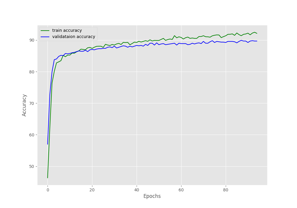
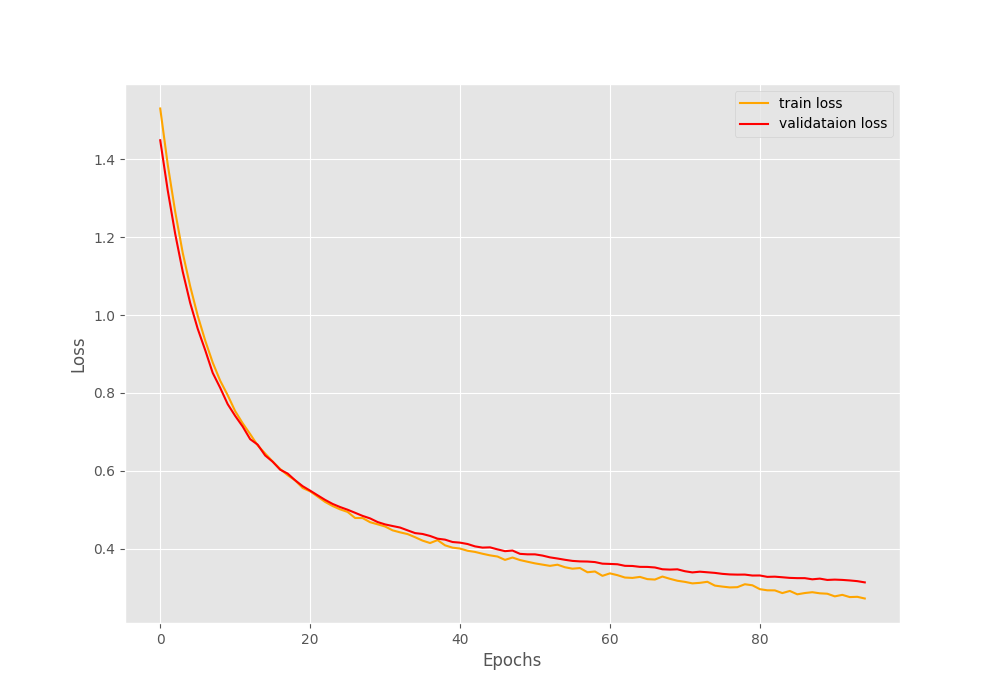
By the end of 95 epochs, we have reached almost 90% validation accuracy and around 0.31 validation loss. From the graphs, it looks like if we apply a learning rate scheduler, we could train even for a few more epochs. Well, that’s for future experiments.

For now, let’s hope that our model has learned well enough to be able to classify entirely new images from the internet.

The Inference

There are five test images in the input/test_data directory, one from each class. We will write the inference script to test our trained model on these images.

The inference code will go into the inference.py script.

Let’s start with importing the modules, constructing the argument parser, defining the computation device, and creating a list containing all the class names.

import torch
import cv2
import torchvision.transforms as transforms
import argparse

from model import build_model

# construct the argument parser
parser = argparse.ArgumentParser()
parser.add_argument('-i', '--input', 
    default='input/test_data/daisy.jpg',
    help='path to the input image')
args = vars(parser.parse_args())

# the computation device
device = 'cpu'

# list containing all the labels
labels = ['daisy', 'dandelion', 'rose', 'sunflower', 'tulip']

We will pass the path to the test image through the command line while executing the script using the --input flag. As we are just inferencing on images, the computation device is cpu.

Load the Trained Model Weights and Define the Transforms

The next code block initializes the ShuffleNetV2 model, loads our custom-trained model weights, and defines the standard transforms required for inference.

# initialize the model and load the trained weights
model = build_model(pretrained=False, fine_tune=False).to(device)
print('[INFO]: Loading custom-trained weights...')
checkpoint = torch.load('outputs/model.pth', map_location=device)
model.load_state_dict(checkpoint['model_state_dict'])
model.eval()

# define preprocess transforms
transform = transforms.Compose([
    transforms.ToPILImage(),
    transforms.Resize(224),
    transforms.ToTensor(),
    transforms.Normalize(
        mean=[0.485, 0.456, 0.406],
        std=[0.229, 0.224, 0.225]
    )
]) 

For the test transforms we are:

• Converting the image to PIL Image format.
• Resizing the 224×224 dimensions.
• Converting the images to tensors.
• And applying normalization.

Read the Image and Carry Out the Inference

Finally, we will read the image from the --input path, carry out the inference, and show the results on the screen.

# read and preprocess the image
image = cv2.imread(args['input'])
# get the ground truth class
gt_class = args['input'].split('/')[-1].split('.')[0]
orig_image = image.copy()
# convert to RGB format
image = cv2.cvtColor(image, cv2.COLOR_BGR2RGB)
image = transform(image)
# add batch dimension
image = torch.unsqueeze(image, 0)
with torch.no_grad():
    outputs = model(image.to(device))
output_label = torch.topk(outputs, 1)
pred_class = labels[int(output_label.indices)]
cv2.putText(orig_image, 
    f"GT: {gt_class}",
    (10, 25),
    cv2.FONT_HERSHEY_SIMPLEX, 
    1, (0, 255, 0), 2, cv2.LINE_AA
)
cv2.putText(orig_image, 
    f"Pred: {pred_class}",
    (10, 55),
    cv2.FONT_HERSHEY_SIMPLEX, 
    1, (0, 0, 255), 2, cv2.LINE_AA
)
print(f"GT: {gt_class}, pred: {pred_class}")
cv2.imshow('Result', orig_image)
cv2.waitKey(0)
cv2.imwrite(f"outputs/{gt_class}.png",
    orig_image)

• After reading the image (line 38), we are extracing the ground truth class from the image path string on line 40.
• We are also keeping a copy of the image for cv2 annotations later on.
• After converting the image to RGB format, we are applying the transform, adding the batch dimension, and passing it through the model.
• We are getting the top 1 output from the outputs and storing the predicted class name in pred_class after mapping the index to the labels list.
• Finally, we are putting the ground truth and predicted class name on the original image, printing the outputs on the terminal, and saving the results to the disk as well.

Let’s execute the infernece.py script and check out the outputs.

Execute inference.py Script

There are five test images. Let’s test each of them.

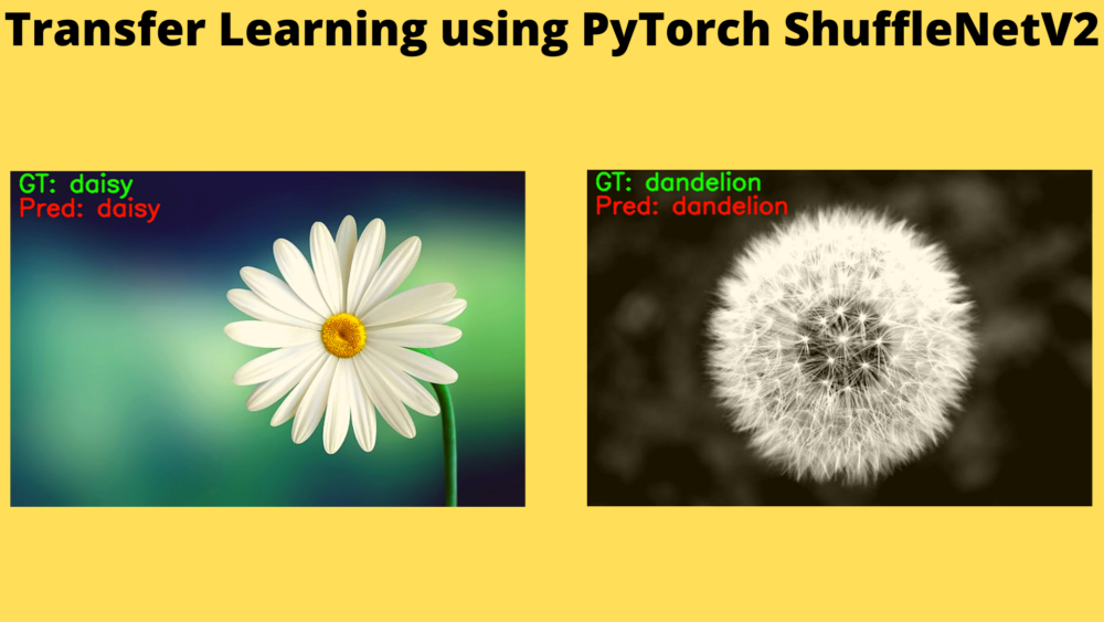
Starting with the daisy.jpg image.

python inference.py --input input/test_data/daisy.jpg 

The following is the output on the terminal.

[INFO]: Not loading pre-trained weights
[INFO]: Freezing hidden layers...
[INFO]: Loading custom-trained weights...
GT: daisy, pred: daisy

As we can see the model is able to predict the class of the flower correctly.

Trying out the dandelion.jpg image.

python inference.py --input input/test_data/dandelion.jpg 

[INFO]: Not loading pre-trained weights
[INFO]: Freezing hidden layers...
[INFO]: Loading custom-trained weights...
GT: dandelion, pred: dandelion

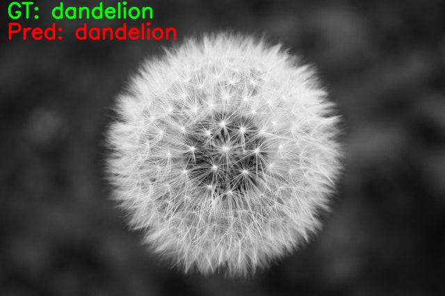
This time also the prediction is correct.

Let’s try out the other three images.

python inference.py --input input/test_data/rose.jpg 

[INFO]: Not loading pre-trained weights
[INFO]: Freezing hidden layers...
[INFO]: Loading custom-trained weights...
GT: rose, pred: rose

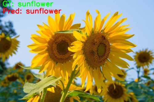
Now, the image of a sunflower.

python inference.py --input input/test_data/sunflower.jpg 

[INFO]: Not loading pre-trained weights
[INFO]: Freezing hidden layers...
[INFO]: Loading custom-trained weights...
GT: sunflower, pred: sunflower

Finally, the image of a tulip.

python inference.py --input input/test_data/tulip.jpg 

[INFO]: Not loading pre-trained weights
[INFO]: Freezing hidden layers...
[INFO]: Loading custom-trained weights...
GT: tulip, pred: tulip

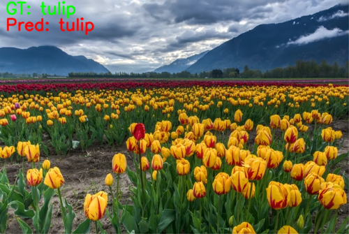
As we can see our model is able to predict all the flower classes correctly. It has learned the features of the five flowers really well.

Summary and Conclusion

In this tutorial, you learned how to use transfer learning to train a PyTorch ShuffleNetV2 model to recognize five different classes of flowers. This project can be taken further by introducing concepts like training for more epochs, applying a learning rate scheduler, and early stopping. I hope that you learned something new from this tutorial.

If you have any doubts, thoughts, or suggestions, please leave them in the comment section. I will surely address them.

You can contact me using the Contact section. You can also find me on LinkedIn, and Twitter.