Using object detection models which are pre-trained on the MS COCO dataset is a common practice in the field of computer vision and deep learning. And that works well most of the time as the MS COCO dataset has 80 classes. This means that all the models which are pre-trained on this dataset, are capable of detecting objects from 80 different categories. This covers objects like persons, cars, trucks, etc. And many of the production level systems use these models for their use case.
But what if we want to detect objects which are not in the MS COCO dataset? Obviously, we have to train our model. Then again, training a model from scratch is not a good idea as we need a lot of data and time for that. Instead, we can use the learned features of the state-of-the-art pre-trained object detection models. And we can then use transfer learning to train on our own dataset.
This has two benefits:
We do not need as much data compared to training from scratch.
The training time reduces by a good margin.
Approach for this Tutorial
In this tutorial, we will follow a similar approach. We will train a custom object detection model using PyTorch Faster RCNN. Basically, we will cover the following points in this tutorial.
We will train a custom object detection model using the pre-trained PyTorch Faster RCNN model.
We will create a simple yet very effective pipeline to fine-tune the PyTorch Faster RCNN model.
After the training completes, we will also carry out inference using new images from the internet that the model has not seen during training or validation.
If you are new to object detection in PyTorch, then I highly recommend going through some of the previous inference tutorials which use the Faster RCNN model. You will have a much better idea after that and also find this tutorial a bit easier to follow.
Note: I hope that this tutorial serves as a good starting point to explore custom object detection using PyTorch for you. If you find the code useful, you are free to use it anyhow you like and even expand it into a larger project.
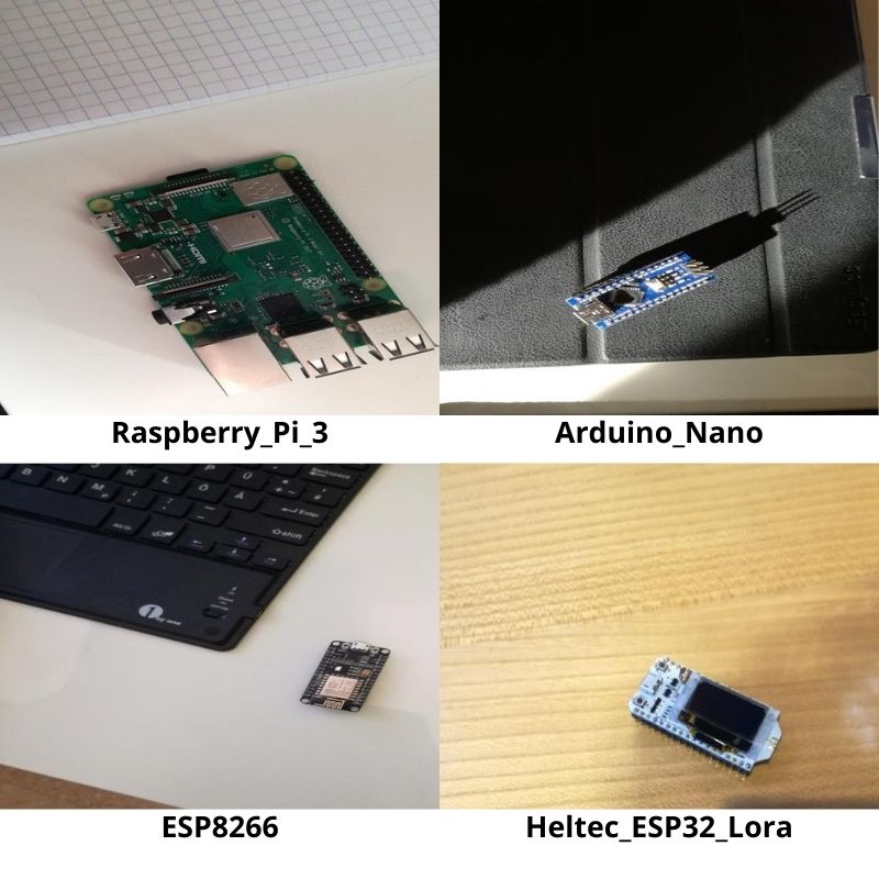
The Microcontroller Detection Dataset
For this custom object detection using the PyTorch Faster RCNN tutorial, we will use the Microcontroller Dataset. This dataset contains images of microcontrollers and microcomputers belonging to 4 different classes. They are:
Arduino_Nano
ESP8266
Raspberry_Pi_3
Heltec_ESP32_Lora
It has 142 training samples and 7 validation samples. Now, this might look very less in the beginning. But in fact, it is just perfect for learning about custom detector training and learning about the training pipeline.
The following is the directory structure of the data.
We have train and test subdirectories that contain the JPG images and corresponding XML files. The XML files contain the information about the corresponding image such as:
We can also see two CSV files. These also contain the same information as the XML files for the training and test images, except in tabular format. But while preparing the PyTorch dataset, we will rely on the XML files.
And just to finish off the exploration of the dataset, here are a few images from the training set.
Figure 1. A few examples from the training set of the microcontroller dataset.
Before moving further, be sure to download the dataset. In the next section, we will see how to structure the project directory along with the dataset.
Directory Structure
As we will be carrying out a custom object detection project, having a simple yet effective directory structure is pretty much important.
After extracting the downloaded dataset, you should have a Microcontroller Detection folder in the parent project directory. This contains the train and test subdirectories which in turn contain the JPG images and XML files.
The src folder contains the Python code files that we need in this tutorial. We will explore these in the coding section later on.
The outputs folder will contain the trained models and the loss graphs which will be generated while training the PyTorch Faster RCNN model.
In the test_data folder we have the images that we will use for inference after training.
And finally, the test_predictions will contain the inference image results.
You will get access to the source code and inference images when downloading the code files for this tutorial.
Required Libraries and Frameworks
For the PyTorch framework, it will be best if you have the latest version, that is PyTorch version 1.9.0 at the time of writing this tutorial. If a new version is out there while you are reading, feel free to install that.
You also need the Albumentations library for image augmentations. This provides very easy methods to apply data augmentations for object detection datasets among many other features as well. It will be best to use whatever latest version is out there. However, this tutorial uses version 1.0.3.
If further on you find that you are missing any other libraries, feel free to install them as you go.
Custom Object Detection using PyTorch Faster RCNN
From this section onward, we will start the coding part of the tutorial.
To get our entire training pipeline ready, we need five Python files.
config.py
datasets.py
utils.py
model.py
engine.py
We will handle each of these Python code files in separate sub-sections.
Creating the Training Configuration File
It is always a good idea to keep the training configuration file separate. This ensures that we need not fiddle around with other parts of the pipeline when wanting to change, for example, the input image size or the number of epochs.
In our case also, we have one such file containing these configurations. The following code will go into the config.py Python file.
import torch

BATCH_SIZE = 4 # increase / decrease according to GPU memeory
RESIZE_TO = 512 # resize the image for training and transforms
NUM_EPOCHS = 100 # number of epochs to train for

DEVICE = torch.device('cuda') if torch.cuda.is_available() else torch.device('cpu')

# training images and XML files directory
TRAIN_DIR = '../Microcontroller Detection/train'
# validation images and XML files directory
VALID_DIR = '../Microcontroller Detection/test'

# classes: 0 index is reserved for background
CLASSES = [
    'background', 'Arduino_Nano', 'ESP8266', 'Raspberry_Pi_3', 'Heltec_ESP32_Lora'
]
NUM_CLASSES = 5

# whether to visualize images after crearing the data loaders
VISUALIZE_TRANSFORMED_IMAGES = False

# location to save model and plots
OUT_DIR = '../outputs'
SAVE_PLOTS_EPOCH = 2 # save loss plots after these many epochs
SAVE_MODEL_EPOCH = 2 # save model after these many epochs
Okay, we have a bit going on in the above code block. Most of these are self-explanatory and the comments should help out as well. Let’s go through a few of the important ones.
Going Through the Above Configurations
RESIZE_TO: This is set to 512. We will resize both, the images and the corresponding bounding boxes to 512 before feeding the images to the augmentations. Resizing has an effect on training time and GPU memory requirements as well. 512 is a good spot for this dataset.
TRAIN_DIR and VALID_DIR: These two are the path to the folders containing the images and the corresponding XML files for the training and validation set. Remember that the images and XML files are in the same directory. That’s how we will write the code as well.
CLASSES: We have 4 classes in total for this dataset. But this list contains an additional background in the beginning. This is because PyTorch Faster RCNN always expects this additional class along with the classes of the dataset. This also makes the NUM_CLASSES equal to 5.
VISUALIZE_TRANSFORMED_IMAGES: If this is set to True, then before the training starts, a transformed image will be visualized on the screen just to check that all the augmentations and the class names are proper. If you do not want that image to pop up, just set it to False.
SAVE_PLOTS_EPOCH and SAVE_MODEL_EPOCH: These two control the interval at which the loss plots and models are saved to OUT_DIR. Also, after training, the final model and final loss plot will always be saved. We will see that later on.
These parameters and hyperparameters control most of the training settings. And once we change them here, we need not change anything else in the rest of the code.
Utility and Helper Functions
When carrying out custom object detection training, we need a lot of utility code and helper functions. Although we don’t have much for our project, still keeping it in a separate Python file is a good idea.
The code for this section will go into the utils.py file.
The following code block contains the import statements and the first class of the Python file.
import albumentations as A
import cv2
import numpy as np

from albumentations.pytorch import ToTensorV2
from config import DEVICE, CLASSES as classes

# this class keeps track of the training and validation loss values...
# ... and helps to get the average for each epoch as well
class Averager:
    def __init__(self):
        self.current_total = 0.0
        self.iterations = 0.0

    def send(self, value):
        self.current_total += value
        self.iterations += 1

    @property
    def value(self):
        if self.iterations == 0:
            return 0
        else:
            return 1.0 * self.current_total / self.iterations

    def reset(self):
        self.current_total = 0.0
        self.iterations = 0.0
In the imports we have albumentations and its modules as we will be defining the training and validation augmentation transforms here. We also have the required variables from the config module.
We have an Averager class. This will help us keep track of the training and validation loss values and also average them for each epoch. We will see its proper usage when writing the training code.
The next code block defines the collate_fn() function.
def collate_fn(batch):
    """
    To handle the data loading as different images may have different number
    of objects and to handle varying size tensors as well.
    """
    return tuple(zip(*batch))
This helps during data loading. In object detection, each image will very likely have a different number of objects and also these objects will give rise to tensors of varying sizes. The collate_fn() function will handle the images and bounding boxes of varying sizes for us without much manual coding.
The Training and Validation Augmentations
We have two functions defining the training and validation transforms.
We have quite a few augmentations for the training set. Note that among others, we also have RandomRotate90 and Flip augmentations. The best part is that albumentations will also handle the orientation of the corresponding bounding boxes when applying these augmentations. This reduces a lot of manual coding. For the validation set, we just convert everything to tensors.
Function to Show Transformed Images
Now, you must be remembering the VISUALIZE_TRANSFORMED_IMAGES variable in config.py. When that value is True, then the following function will be executed to show the transformed images just before the training begins. In simple words, these are the images after augmentations, which the model actually sees during training.
def show_tranformed_image(train_loader):
    """
    This function shows the transformed images from the `train_loader`.
    Helps to check whether the tranformed images along with the corresponding
    labels are correct or not.
    Only runs if `VISUALIZE_TRANSFORMED_IMAGES = True` in config.py.
    """
    if len(train_loader) > 0:
        for i in range(1):
            images, targets = next(iter(train_loader))
            images = list(image.to(DEVICE) for image in images)
            targets = [{k: v.to(DEVICE) for k, v in t.items()} for t in targets]
            boxes = targets[i]['boxes'].cpu().numpy().astype(np.int32)
            sample = images[i].permute(1, 2, 0).cpu().numpy()
            for box in boxes:
                cv2.rectangle(sample,
                            (box[0], box[1]),
                            (box[2], box[3]),
                            (0, 0, 255), 2)
            cv2.imshow('Transformed image', sample)
            cv2.waitKey(0)
            cv2.destroyAllWindows()
This completes the code that we need for the utils.py file.
Preparing the Dataset
This section is going to be pretty important as we will be writing the code to prepare the MicrocontrollerDataset.
The main thing we want to understand here is the code in the MicrocontrollerDataset class.
We will write the dataset preparation code in datasets.py file.
Before we get into that, let’s import all the required modules and libraries.
import torch
import cv2
import numpy as np
import os
import glob as glob

from xml.etree import ElementTree as et
from config import CLASSES, RESIZE_TO, TRAIN_DIR, VALID_DIR, BATCH_SIZE
from torch.utils.data import Dataset, DataLoader
from utils import collate_fn, get_train_transform, get_valid_transform
We have imported the required parameters from the config and utils modules. We also need the DataLoader and Dataset classes from the torch.utils.data.
The MicrocontrollerDataset Class
The MicrocontrollerDataset class is going to be a bit large code block. Let’s put all that code in the next block to maintain continuity and indentation, then we will get to the explanation part.
# the dataset class
class MicrocontrollerDataset(Dataset):
    def __init__(self, dir_path, width, height, classes, transforms=None):
        self.transforms = transforms
        self.dir_path = dir_path
        self.height = height
        self.width = width
        self.classes = classes

        # get all the image paths in sorted order
        self.image_paths = glob.glob(f"{self.dir_path}/*.jpg")
        self.all_images = [image_path.split('/')[-1] for image_path in self.image_paths]
        self.all_images = sorted(self.all_images)

    def __getitem__(self, idx):
        # capture the image name and the full image path
        image_name = self.all_images[idx]
        image_path = os.path.join(self.dir_path, image_name)

        # read the image
        image = cv2.imread(image_path)
        # convert BGR to RGB color format
        image = cv2.cvtColor(image, cv2.COLOR_BGR2RGB).astype(np.float32)
        image_resized = cv2.resize(image, (self.width, self.height))
        image_resized /= 255.0

        # capture the corresponding XML file for getting the annotations
        annot_filename = image_name[:-4] + '.xml'
        annot_file_path = os.path.join(self.dir_path, annot_filename)

        boxes = []
        labels = []
        tree = et.parse(annot_file_path)
        root = tree.getroot()

        # get the height and width of the image
        image_width = image.shape[1]
        image_height = image.shape[0]

        # box coordinates for xml files are extracted and corrected for image size given
        for member in root.findall('object'):
            # map the current object name to `classes` list to get...
            # ... the label index and append to `labels` list
            labels.append(self.classes.index(member.find('name').text))

            # xmin = left corner x-coordinates
            xmin = int(member.find('bndbox').find('xmin').text)
            # xmax = right corner x-coordinates
            xmax = int(member.find('bndbox').find('xmax').text)
            # ymin = left corner y-coordinates
            ymin = int(member.find('bndbox').find('ymin').text)
            # ymax = right corner y-coordinates
            ymax = int(member.find('bndbox').find('ymax').text)

            # resize the bounding boxes according to the...
            # ... desired `width`, `height`
            xmin_final = (xmin/image_width)*self.width
            xmax_final = (xmax/image_width)*self.width
            ymin_final = (ymin/image_height)*self.height
            yamx_final = (ymax/image_height)*self.height

            boxes.append([xmin_final, ymin_final, xmax_final, yamx_final])

        # bounding box to tensor
        boxes = torch.as_tensor(boxes, dtype=torch.float32)
        # area of the bounding boxes
        area = (boxes[:, 3] - boxes[:, 1]) * (boxes[:, 2] - boxes[:, 0])
        # no crowd instances
        iscrowd = torch.zeros((boxes.shape[0],), dtype=torch.int64)
        # labels to tensor
        labels = torch.as_tensor(labels, dtype=torch.int64)

        # prepare the final `target` dictionary
        target = {}
        target["boxes"] = boxes
        target["labels"] = labels
        target["area"] = area
        target["iscrowd"] = iscrowd
        image_id = torch.tensor([idx])
        target["image_id"] = image_id

        # apply the image transforms
        if self.transforms:
            sample = self.transforms(image = image_resized,
                                     bboxes = target['boxes'],
                                     labels = labels)
            image_resized = sample['image']
            target['boxes'] = torch.Tensor(sample['bboxes'])

        return image_resized, target

    def __len__(self):
        return len(self.all_images)
We will go through each of the methods.
__init__() Method
It accepts five parameters that we initialize just after declaring the method.
self.transforms: Either the training or the validation transforms. These hold the information about the image augmentations we want to carry out.
self.dir_path: Path to the directory containing either the training or validation images and XML files.
self.height and self.width: Dimensions to resize the images to. We also change the respective bounding box coordinate values accordingly.
self.classes: List containing all the class names.
The next three lines of code create the self.all_images list which contains all the image names in sorted order. We need these to read the images later on.
__getitem__ Method
After getting the current image path on line 28, we read the image on line 31. Then we convert the color format from BGR to RGB, resize it to the required height and width, and scale the image pixels.
Starting from line 38, we read the corresponding XML file for the image. We have the labels and boxes lists to store the bounding box coordinates and labels for the current image.
Starting from line 51, we parse through the XML file. On line 54, we append the class name to labels. From line 57 till 63, we extract the bounding box coordinates. Then we resize those bounding boxes to the desired to height and width (lines 67 to 70). And then we append the resized bounding boxes to the boxes list.
We convert the boxes and labels to tensors on lines 75 and 81 respectively. We also calculate the area of the bounding boxes and none of our data is labeled as iscrowd.
We have a target dictionary where we store all the information collected till now.
Then we apply the transforms to the image and return the resized image and the target dictionary.
Creating the Data Loaders
The next step is to create the training and validation datasets and data loaders.
# prepare the final datasets and data loaders
train_dataset = MicrocontrollerDataset(TRAIN_DIR, RESIZE_TO, RESIZE_TO, CLASSES, get_train_transform())
valid_dataset = MicrocontrollerDataset(VALID_DIR, RESIZE_TO, RESIZE_TO, CLASSES, get_valid_transform())
train_loader = DataLoader(
    train_dataset,
    batch_size=BATCH_SIZE,
    shuffle=True,
    num_workers=0,
    collate_fn=collate_fn
)
valid_loader = DataLoader(
    valid_dataset,
    batch_size=BATCH_SIZE,
    shuffle=False,
    num_workers=0,
    collate_fn=collate_fn
)
print(f"Number of training samples: {len(train_dataset)}")
print(f"Number of validation samples: {len(valid_dataset)}\n")
The above code block defines the training and validation datasets and also the iterable data loaders. Note that the num_workers has been set to 0. If you are on any of the Linux systems and trying to execute the code locally, try using a value of 2 or above. This will likely decrease the data fetching time.
We are also printing the number of training and validation samples that we have.
We just have one final block of code for this Python file. Let’s check it out.
# execute datasets.py using Python command from Terminal...
# ... to visualize sample images
# USAGE: python datasets.py
if __name__ == '__main__':
    # sanity check of the Dataset pipeline with sample visualization
    dataset = MicrocontrollerDataset(
        TRAIN_DIR, RESIZE_TO, RESIZE_TO, CLASSES
    )
    print(f"Number of training images: {len(dataset)}")

    # function to visualize a single sample
    def visualize_sample(image, target):
        box = target['boxes'][0]
        label = CLASSES[target['labels']]
        cv2.rectangle(
            image,
            (int(box[0]), int(box[1])), (int(box[2]), int(box[3])),
            (0, 255, 0), 1
        )
        cv2.putText(
            image, label, (int(box[0]), int(box[1]-5)),
            cv2.FONT_HERSHEY_SIMPLEX, 0.7, (0, 0, 255), 2
        )
        cv2.imshow('Image', image)
        cv2.waitKey(0)

    NUM_SAMPLES_TO_VISUALIZE = 5
    for i in range(NUM_SAMPLES_TO_VISUALIZE):
        image, target = dataset[i]
        visualize_sample(image, target)
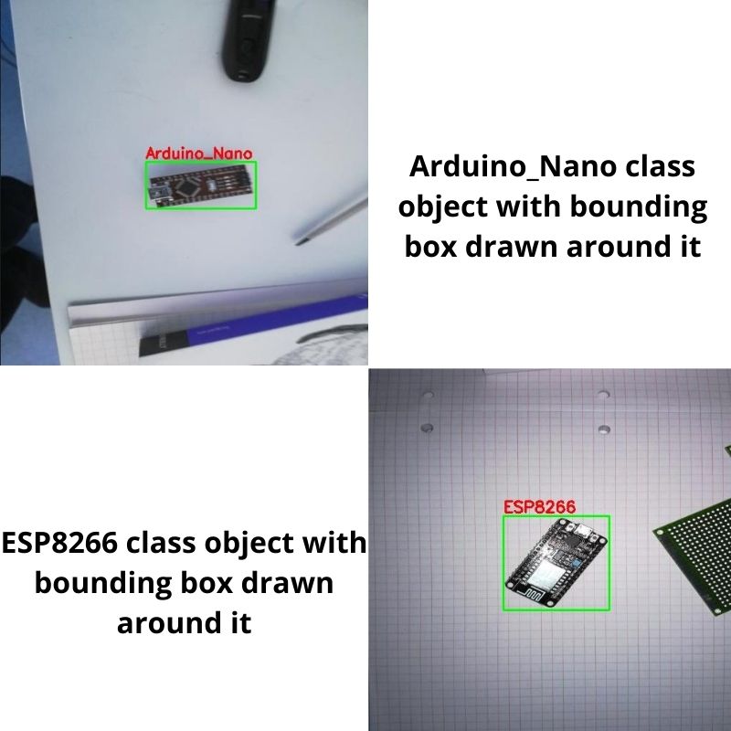
The above code block will only be executed if we directly run the datasets.py file from the terminal/command line. This is just like a sanity check on whether all the data creation pipeline is working correctly or not. If everything is fine, then you should see a few images with the bounding boxes drawn on the objects and also with the labels. You can control the number of images to visualize using the NUM_SAMPLES_TO_VISUALIZE on line 149. You can press the q key on the keyboard to exit the visualizations.
Following are a few examples of those visualizations.
Figure 2. A few microcontroller images with their bounding boxes.
We have completed all the code that we need to prepare the datasets for custom object detection using PyTorch Faster RCNN.
Let’s move on to the next Python file.
The Faster RCNN Model
Here, we will create the Faster RCNN model. This will be really simple as PyTorch already provides a pretrained model. We just need to change the head of the network according to the number of classes in our dataset.
The following code will go into the model.py file.
import torchvision

from torchvision.models.detection.faster_rcnn import FastRCNNPredictor

def create_model(num_classes):

    # load Faster RCNN pre-trained model
    model = torchvision.models.detection.fasterrcnn_resnet50_fpn(pretrained=True)

    # get the number of input features
    in_features = model.roi_heads.box_predictor.cls_score.in_features
    # define a new head for the detector with required number of classes
    model.roi_heads.box_predictor = FastRCNNPredictor(in_features, num_classes)

    return model
On line 8, we load the pretrained Faster RCNN model with the ResNet50 FPN backbone. Then on line 11, we get the number of input features. For this particular model, it is 1024.
Finally, we change the head of the Faster RCNN detector according to the in_features and the number of classes.
This is all we need to prepare the PyTorch Faster RCNN model.
The Executable Training Script
It’s time to write the Python script that will run all the code we have been writing till now. This is the final Python code file before we begin custom object detection training using Pytorch Faster RCNN.
This is an executable script. All this code will go into the engine.py file.
The first code block contains all the import statements.
from config import DEVICE, NUM_CLASSES, NUM_EPOCHS, OUT_DIR
from config import VISUALIZE_TRANSFORMED_IMAGES
from config import SAVE_PLOTS_EPOCH, SAVE_MODEL_EPOCH
from model import create_model
from utils import Averager
from tqdm.auto import tqdm
from datasets import train_loader, valid_loader

import torch
import matplotlib.pyplot as plt
import time

plt.style.use('ggplot')
We have all the required imports that we need for further code. Do take a look to check all the modules that we are importing.
The Training Function
Next, we have the training function to carry out the object detection forward and backward pass.
# function for running training iterations
def train(train_data_loader, model):
    print('Training')
    global train_itr
    global train_loss_list

     # initialize tqdm progress bar
    prog_bar = tqdm(train_data_loader, total=len(train_data_loader))

    for i, data in enumerate(prog_bar):
        optimizer.zero_grad()
        images, targets = data

        images = list(image.to(DEVICE) for image in images)
        targets = [{k: v.to(DEVICE) for k, v in t.items()} for t in targets]

        loss_dict = model(images, targets)

        losses = sum(loss for loss in loss_dict.values())
        loss_value = losses.item()
        train_loss_list.append(loss_value)

        train_loss_hist.send(loss_value)

        losses.backward()
        optimizer.step()

        train_itr += 1

        # update the loss value beside the progress bar for each iteration
        prog_bar.set_description(desc=f"Loss: {loss_value:.4f}")
    return train_loss_list
The train() function accepts the training data loader and the model.
If you observe, on lines 17 and 18, we are accessing the train_itr and train_loss_list variables globally. These are two lists that keep on storing the number of training iterations and the training loss for each iteration till the end of training. This will be very useful for plotting loss graphs later on.
On line 21, we are defining a progress bar, prog_bar using the train_data_loader. Along with showing a progress bar for the passing iterations, the loss values for each batch will keep on updating beside it. This is very useful when a single epoch takes a long time to complete as we can see the loss updates for each batch. The displaying of the updated loss is done on line 44.
Then we have the for loop iterating over the batches. First, we extract the images and targets and load them onto the computation device of choice.
The forward pass happens on line 30.
Then we sum the losses and append the current iteration’s loss value to train_loss_list list. We also send the current loss value to train_loss_hist of the Averager class.
Then we backpropagate the gradients and update parameters.
We just return the train_loss_list for plotting the loss graph.
The Validation Function
The validation function will be very similar to the training function except:
We do not do backpropagation.
We do not update any parameters.
# function for running validation iterations
def validate(valid_data_loader, model):
    print('Validating')
    global val_itr
    global val_loss_list

    # initialize tqdm progress bar
    prog_bar = tqdm(valid_data_loader, total=len(valid_data_loader))

    for i, data in enumerate(prog_bar):
        images, targets = data

        images = list(image.to(DEVICE) for image in images)
        targets = [{k: v.to(DEVICE) for k, v in t.items()} for t in targets]

        with torch.no_grad():
            loss_dict = model(images, targets)

        losses = sum(loss for loss in loss_dict.values())
        loss_value = losses.item()
        val_loss_list.append(loss_value)

        val_loss_hist.send(loss_value)

        val_itr += 1

        # update the loss value beside the progress bar for each iteration
        prog_bar.set_description(desc=f"Loss: {loss_value:.4f}")
    return val_loss_list
Similar to the training function, we are returning the val_loss_list here.
The Main Code
Now, we have reached the main code that will run all of the above. Let’s write the code first.
if __name__ == '__main__':
    # initialize the model and move to the computation device
    model = create_model(num_classes=NUM_CLASSES)
    model = model.to(DEVICE)
    # get the model parameters
    params = [p for p in model.parameters() if p.requires_grad]
    # define the optimizer
    optimizer = torch.optim.SGD(params, lr=0.001, momentum=0.9, weight_decay=0.0005)

    # initialize the Averager class
    train_loss_hist = Averager()
    val_loss_hist = Averager()
    train_itr = 1
    val_itr = 1
    # train and validation loss lists to store loss values of all...
    # ... iterations till ena and plot graphs for all iterations
    train_loss_list = []
    val_loss_list = []

    # name to save the trained model with
    MODEL_NAME = 'model'

    # whether to show transformed images from data loader or not
    if VISUALIZE_TRANSFORMED_IMAGES:
        from utils import show_tranformed_image
        show_tranformed_image(train_loader)

    # start the training epochs
    for epoch in range(NUM_EPOCHS):
        print(f"\nEPOCH {epoch+1} of {NUM_EPOCHS}")

        # reset the training and validation loss histories for the current epoch
        train_loss_hist.reset()
        val_loss_hist.reset()

        # create two subplots, one for each, training and validation
        figure_1, train_ax = plt.subplots()
        figure_2, valid_ax = plt.subplots()

        # start timer and carry out training and validation
        start = time.time()
        train_loss = train(train_loader, model)
        val_loss = validate(valid_loader, model)
        print(f"Epoch #{epoch} train loss: {train_loss_hist.value:.3f}")
        print(f"Epoch #{epoch} validation loss: {val_loss_hist.value:.3f}")
        end = time.time()
        print(f"Took {((end - start) / 60):.3f} minutes for epoch {epoch}")

        if (epoch+1) % SAVE_MODEL_EPOCH == 0: # save model after every n epochs
            torch.save(model.state_dict(), f"{OUT_DIR}/model{epoch+1}.pth")
            print('SAVING MODEL COMPLETE...\n')

        if (epoch+1) % SAVE_PLOTS_EPOCH == 0: # save loss plots after n epochs
            train_ax.plot(train_loss, color='blue')
            train_ax.set_xlabel('iterations')
            train_ax.set_ylabel('train loss')
            valid_ax.plot(val_loss, color='red')
            valid_ax.set_xlabel('iterations')
            valid_ax.set_ylabel('validation loss')
            figure_1.savefig(f"{OUT_DIR}/train_loss_{epoch+1}.png")
            figure_2.savefig(f"{OUT_DIR}/valid_loss_{epoch+1}.png")
            print('SAVING PLOTS COMPLETE...')

        if (epoch+1) == NUM_EPOCHS: # save loss plots and model once at the end
            train_ax.plot(train_loss, color='blue')
            train_ax.set_xlabel('iterations')
            train_ax.set_ylabel('train loss')
            valid_ax.plot(val_loss, color='red')
            valid_ax.set_xlabel('iterations')
            valid_ax.set_ylabel('validation loss')
            figure_1.savefig(f"{OUT_DIR}/train_loss_{epoch+1}.png")
            figure_2.savefig(f"{OUT_DIR}/valid_loss_{epoch+1}.png")

            torch.save(model.state_dict(), f"{OUT_DIR}/model{epoch+1}.pth")

        plt.close('all')
A lot is going on in the above code block. But most of it is self-explanatory. Let’s check out all the important parts.
We are using the SGD optimizer with a learning rate of 0.001 and momentum on 0.9.
We can also see the initializations of the train_loss_hist, val_loss_hist, train_loss_list, and val_loss_list that we observed in the training and validation functions.
On line 98, we check whether to show the transformed images from the data loader or not.
We start the training epoch iteration from line 103.
We call the train() and validate() functions on lines 116 and 117 respectively.
After printing the metrics for each epoch, we check whether we should save the current model and loss graphs depending on the SAVE_MODEL_EPOCH and SAVE_PLOTS_EPOCH intervals.
On line 138, we do a final saving of the loss graphs and the trained model after all the epochs are complete.
If you wish, take a bit more time to understand the above code. The code may not look very optimal but it surely is simple. Let’s keep things simple for now in this custom object detection pipeline.
Execute engine.py for Custom Object Detection using PyTorch Faster RCNN
Now we are all set to start the training. Please note that we are training for 100 epochs. So, if you are training on your own system, it might take some time to complete.
Open your terminal/command line from in the src directory and execute the following command.
python engine.py
The following are the sample outputs.
Number of training samples: 142
Number of validation samples: 7

Downloading: "https://download.pytorch.org/models/fasterrcnn_resnet50_fpn_coco-258fb6c6.pth" to /root/.cache/torch/hub/checkpoints/fasterrcnn_resnet50_fpn_coco-258fb6c6.pth
100%|████████████████████████████████████████| 160M/160M [00:01<00:00, 88.1MB/s]

EPOCH 1 of 100
Training
Loss: 0.2074: 100%|█████████████████████████████| 36/36 [00:16<00:00,  2.21it/s]
Validating
Loss: 0.3287: 100%|███████████████████████████████| 2/2 [00:00<00:00,  3.62it/s]
Epoch #0 train loss: 0.525
Epoch #0 validation loss: 0.314
Took 0.281 minutes for epoch 0

EPOCH 2 of 100
Training
Loss: 0.3073: 100%|█████████████████████████████| 36/36 [00:15<00:00,  2.27it/s]
Validating
Loss: 0.2832: 100%|███████████████████████████████| 2/2 [00:00<00:00,  4.00it/s]
Epoch #1 train loss: 0.320
Epoch #1 validation loss: 0.275
Took 0.273 minutes for epoch 1
SAVING MODEL COMPLETE...

SAVING PLOTS COMPLETE...
...
EPOCH 99 of 100
Training
Loss: 0.0352: 100%|█████████████████████████████| 36/36 [00:16<00:00,  2.23it/s]
Validating
Loss: 0.0394: 100%|███████████████████████████████| 2/2 [00:00<00:00,  3.93it/s]
Epoch #98 train loss: 0.029
Epoch #98 validation loss: 0.044
Took 0.277 minutes for epoch 98

EPOCH 100 of 100
Training
Loss: 0.0533: 100%|█████████████████████████████| 36/36 [00:16<00:00,  2.24it/s]
Validating
Loss: 0.0409: 100%|███████████████████████████████| 2/2 [00:00<00:00,  3.89it/s]
Epoch #99 train loss: 0.028
Epoch #99 validation loss: 0.049
Took 0.276 minutes for epoch 99
SAVING MODEL COMPLETE...

SAVING PLOTS COMPLETE...
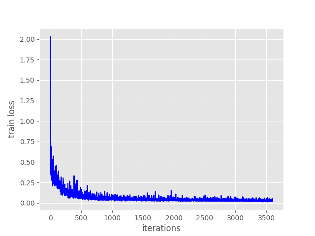
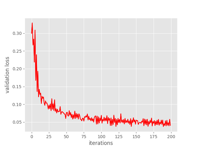
And the following are training and validation loss graphs after the final epoch.
Figure 3. Training loss after training the custom PyTorch Faster RCNN object detection model for 100 epochs.
Figure 4. Validation loss after training the custom PyTorch Faster RCNN object detection model for 100 epochs.
From the graphs, it looks like the training loss plateaued after iteration 1500. But the validation loss was decreasing till the end of training. This means that the model was still learning. Maybe training for even longer would have helped.
Let’s hope that our model has learned enough to perform well on unseen images. That we will get to know after running the inference.
Running Inference using the Trained Faster RCNN Model
The inference script is going to be pretty straightforward. It does not have any dependency on any of the other scripts, we just need to load the trained model.
The inference code will go into the inference.py script.
Let’s import the required modules and load the trained model as well.
import numpy as np
import cv2
import torch
import glob as glob

from model import create_model

# set the computation device
device = torch.device('cuda') if torch.cuda.is_available() else torch.device('cpu')
# load the model and the trained weights
model = create_model(num_classes=5).to(device)
model.load_state_dict(torch.load(
    '../outputs/model100.pth', map_location=device
))
model.eval()
We are using the model weights from the final epoch, that is model100.pth.
The next code block defines the test image directory, the classes, and the detection threshold.
# directory where all the images are present
DIR_TEST = '../test_data'
test_images = glob.glob(f"{DIR_TEST}/*")
print(f"Test instances: {len(test_images)}")

# classes: 0 index is reserved for background
CLASSES = [
    'background', 'Arduino_Nano', 'ESP8266', 'Raspberry_Pi_3', 'Heltec_ESP32_Lora'
]

# define the detection threshold...
# ... any detection having score below this will be discarded
detection_threshold = 0.8
The test_data directory contains all the images that we want to run inference on. All the image paths are stored in test_images. And the detection threshold is 0.8. Any detection that has a score below 0.8 will be discarded.
Looping Over the Image Paths and Carrying Out Inference
Let’s loop over all the image paths at once and carry out the inference.
for i in range(len(test_images)):
    # get the image file name for saving output later on
    image_name = test_images[i].split('/')[-1].split('.')[0]
    image = cv2.imread(test_images[i])
    orig_image = image.copy()
    # BGR to RGB
    image = cv2.cvtColor(orig_image, cv2.COLOR_BGR2RGB).astype(np.float32)
    # make the pixel range between 0 and 1
    image /= 255.0
    # bring color channels to front
    image = np.transpose(image, (2, 0, 1)).astype(np.float)
    # convert to tensor
    image = torch.tensor(image, dtype=torch.float).cuda()
    # add batch dimension
    image = torch.unsqueeze(image, 0)
    with torch.no_grad():
        outputs = model(image)

    # load all detection to CPU for further operations
    outputs = [{k: v.to('cpu') for k, v in t.items()} for t in outputs]
    # carry further only if there are detected boxes
    if len(outputs[0]['boxes']) != 0:
        boxes = outputs[0]['boxes'].data.numpy()
        scores = outputs[0]['scores'].data.numpy()
        # filter out boxes according to `detection_threshold`
        boxes = boxes[scores >= detection_threshold].astype(np.int32)
        draw_boxes = boxes.copy()
        # get all the predicited class names
        pred_classes = [CLASSES[i] for i in outputs[0]['labels'].cpu().numpy()]

        # draw the bounding boxes and write the class name on top of it
        for j, box in enumerate(draw_boxes):
            cv2.rectangle(orig_image,
                        (int(box[0]), int(box[1])),
                        (int(box[2]), int(box[3])),
                        (0, 0, 255), 2)
            cv2.putText(orig_image, pred_classes[j],
                        (int(box[0]), int(box[1]-5)),
                        cv2.FONT_HERSHEY_SIMPLEX, 0.7, (0, 255, 0),
                        2, lineType=cv2.LINE_AA)

        cv2.imshow('Prediction', orig_image)
        cv2.waitKey(1)
        cv2.imwrite(f"../test_predictions/{image_name}.jpg", orig_image,)
    print(f"Image {i+1} done...")
    print('-'*50)

print('TEST PREDICTIONS COMPLETE')
cv2.destroyAllWindows()
We are doing the forward pass on line 45 within the torch.no_grad() context manager. First, we move all the detection outputs to the CPU on line 48.
Then, we only move further if there are any detections (line 50). On line 54, we filter out the boxes having detection scores below 0.8. The pred_classes list contains the class names of all the detected objects.
Starting from line 60, we draw the bounding boxes around the objects on a copy of the original image. We also put the class name text on top of the bounding boxes. The code will automatically loop over all the images and just show each image for 1 millisecond before moving on to the next
Execute inference.py
Execute inference.py from the src directory using the following command.
python inference.py
You should see the following output on the terminal.
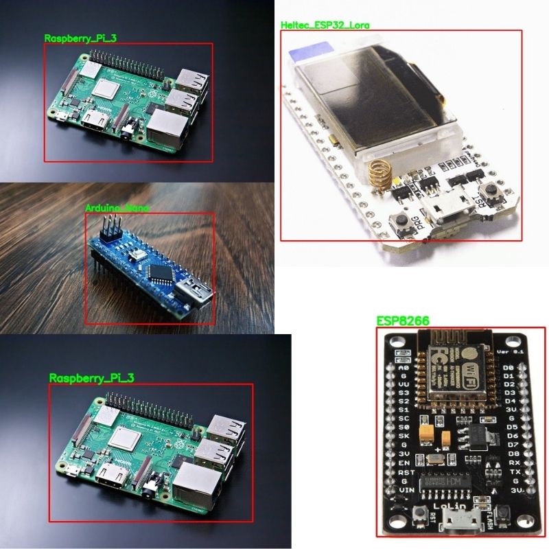
There were five images in the test_data directory. 4 images were from each of the classes and one image had two objects. The file names match the ground truth class names so that we can compare easily.
Let’s check out the predictions. The following image shows all the predictions.
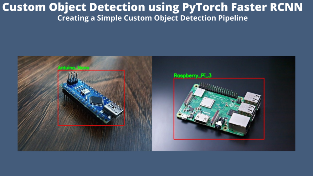
Figure 5. Inference results for custom object detection using PyTorch Faster RCNN.
Interestingly, our custom-trained model is detecting all the classes correctly. The bounding boxes also look pretty tight around the objects. This is a good sign indicating that the model has been trained well.
Further Improvement
You can take this project further by adding more classes for the microcontrollers. Maybe add images and classes for Raspberry Pi 4 as well making the dataset considerably challenging. If you try any new things, let others know in the comment section. I hope that this tutorial provides you with a good initial pipeline to carry out many interesting object detection projects using the Faster RCNN model.
Summary and Conclusion
In this tutorial, you learned how to carry out custom object detection training using the PyTorch Faster RCNN model. We set up a simple pipeline for Faster RCNN object detection training which can be changed and scaled according to requirements. We also used this pipeline to train a custom detector to detect microcontrollers in images.
I hope that you learned something new in this tutorial. If you have any doubts, thoughts, or suggestions, please leave them in the comment section. I will surely address them.
You can contact me using the Contact section. You can also find me on LinkedIn, and X.
Hello Faisal. Replying to your question “Can you please tell me the dataset format of that tutorial” here as the below thread did not allow any more replies. The dataset should be in Pascal VOC XML format.
Hello Jaiyesh. Yes, the pipeline works for multiple objects in an image. Regarding the mAP thing, tomorrow a brand new post for object detection using Faster RCNN will be out. It is a much-improved pipeline with mAP metrics, options for adding different models, etc. Please have a look at that one. It is also part of the traffic sign recognition and detection series which will contain three more posts in the upcoming weeks.
Hello. Sorry to hear that you are having issues. Please let me know your browser. Also, in the meantime, please try to download from another browser. Another alternative is that if you can provide me with your email, I can send you the code directly if that works for you.
Please let me know your thoughts.
I have trained the model but the trained model haven’t been able to predict any object and classes after saving and loading it in interface.py. i have used my own custom dataset.Should i trained more epoch?
God bless you Sir, for work you have done. I have explored several web pages in order to implement Faster RCNN with ResNet or ResNext backbone. But this is definitely best implementation tutorial about Faster RCNN.
Excellent. What a fantastic work Sir!
I really need these materials.
I have a question. Do you have any post about modifying Faster-RCNN ? like adding attention to them, adding branch and … ? or do you know some other sites that contain such things?
Thank you Sir
Hello Rohollah. Thank you for your appreciation.
Currently, I have posts on adding different backbones to the Faster RCNN model. But not about adding attention. Hopefully, I can do that sometime in the near future. In the meantime, you can surely look at these posts for adding different backbones.
Hi Sovit.
Actually I know how to use different backbones with Faster-RCNN, Thank you anyway.
I’m eagerly waiting for your posts about adding attention to Faster-RCNN and so on.
Good luck Sovit.
Hi Sovit, very nice tutorial. I was able to reproduce it without many problems. Quite different to TensorFlow object detection API actually. Thanks a lot.
I trained only for 5 epochs for testing but it still works with a lower detection threshold during inference. However, I would suggest to implement non maximum suppression to filter overlapping detections during inference. This code here for instance works perfectly fine with your code. (https://towardsdatascience.com/non-maxima-suppression-139f7e00f0b5)
Best regards
Hello Marc. I am glad that you find the post helpful.
Regarding the non-maximum suppression part, I think that the Faster RCNN model already applies that as part of the model. We just need to tweak the detection threshold to filter out the final false positives. Also, training for longer will surely help.
Let me know if you have questions further.
Hi Sovit, your turtorial is amazing.
I’m using this for my thesis but i’m not sure about a thing.
Could you please clarify why you don’t resize the image when inferencing? If we start with rectangular images, it even changes the ratio of it during training.
Thanks for your time.
Hello Niccolo.
Generally, for Faster RCNN inference we don’t need to resize the images. Faster RCNN already resizes the images according to a certain ration internally. It does so during training also. But during training, as we are creating data loaders, it expects the images to be of the same size. So, we resize them during training.
But you can surely give it a try to resize the images during inference as well.
Thanks for the answer, i should mention that i used your code on a custom dataset. In that case i found that if i resize the image during inference, it gave better result. i think it’s because during training i was turning rectangular images into a square shape, modifing the ratio of the image.
I think you are on the right path. Thank you for mentioning this,
By the way, I have created a big and easy-to-use library for training Faster RCNN models. Along with the resize correction, there are many other logging utilities, resuming training, etc. in this one. I think you will find it useful. https://github.com/sovit-123/fasterrcnn-pytorch-training-pipeline
I have already trained the model, and now I am confused about how to find the mAP, recall and precision. Looking at the comments, I came to know about another post, however it is already late as my model is already trained.
Is there any way to find the mAP, precision and recall with the model weight model300.pth which is trained based on this article?
Thank you
I think the download link may be broken for the orange “Download the Source Code for this Tutorial”. I can’t click on either in this article but I can click on the same button for other articles.
Hello Jyothsna. Can you please elaborate a bit more on the use case? I guess that you are trying to understand how to detect occluded faces. Are you working with fully or partially occluded faces?
Hi Sovit, very nice tutorial.I have trained the model for 8 epochs using other dataset , but always predicts the same class .
and how i can calcul mAP, precision and recall with the model.
Traceback (most recent call last):
File “/Users/ziemian/Code/bt/src/model.py”, line 60, in
outputs = model(images, targets)
File “/Users/ziemian/Code/python-venvs/deepl/lib/python3.10/site-packages/torch/nn/modules/module.py”, line 1518, in _wrapped_call_impl
return self._call_impl(*args, **kwargs)
File “/Users/ziemian/Code/python-venvs/deepl/lib/python3.10/site-packages/torch/nn/modules/module.py”, line 1527, in _call_impl
return forward_call(*args, **kwargs)
File “/Users/ziemian/Code/python-venvs/deepl/lib/python3.10/site-packages/torchvision/models/detection/generalized_rcnn.py”, line 105, in forward
detections, detector_losses = self.roi_heads(features, proposals, images.image_sizes, targets)
File “/Users/ziemian/Code/python-venvs/deepl/lib/python3.10/site-packages/torch/nn/modules/module.py”, line 1518, in _wrapped_call_impl
return self._call_impl(*args, **kwargs)
File “/Users/ziemian/Code/python-venvs/deepl/lib/python3.10/site-packages/torch/nn/modules/module.py”, line 1527, in _call_impl
return forward_call(*args, **kwargs)
File “/Users/ziemian/Code/python-venvs/deepl/lib/python3.10/site-packages/torchvision/models/detection/roi_heads.py”, line 755, in forward
proposals, matched_idxs, labels, regression_targets = self.select_training_samples(proposals, targets)
File “/Users/ziemian/Code/python-venvs/deepl/lib/python3.10/site-packages/torchvision/models/detection/roi_heads.py”, line 649, in select_training_samples
matched_idxs, labels = self.assign_targets_to_proposals(proposals, gt_boxes, gt_labels)
File “/Users/ziemian/Code/python-venvs/deepl/lib/python3.10/site-packages/torchvision/models/detection/roi_heads.py”, line 588, in assign_targets_to_proposals
labels_in_image = gt_labels_in_image[clamped_matched_idxs_in_image]
IndexError: index 1 is out of bounds for dimension 0 with size 1
It’s kind of hard say exactly what the issue may be. But it seems like ground truth issue. It looks like there is either bounding box or label annotation missing in the dataset.
I’m getting this error when I try to train with a dataset that has multiple labels/boundboxes for one image. Can anyone help me?
Traceback (most recent call last):
File “engine.py”, line 122, in
train_loss = train(train_loader, model)
File “engine.py”, line 25, in train
for i, data in enumerate(prog_bar):
File “/usr/local/lib/python3.8/dist-packages/tqdm/std.py”, line 1182, in __iter__
for obj in iterable:
File “/usr/local/lib/python3.8/dist-packages/torch/utils/data/dataloader.py”, line 633, in __next__
data = self._next_data()
File “/usr/local/lib/python3.8/dist-packages/torch/utils/data/dataloader.py”, line 677, in _next_data
data = self._dataset_fetcher.fetch(index) # may raise StopIteration
File “/usr/local/lib/python3.8/dist-packages/torch/utils/data/_utils/fetch.py”, line 51, in fetch
data = [self.dataset[idx] for idx in possibly_batched_index]
File “/usr/local/lib/python3.8/dist-packages/torch/utils/data/_utils/fetch.py”, line 51, in
data = [self.dataset[idx] for idx in possibly_batched_index]
File “/OBJ_DETECT_PIPELINE/src/datasets.py”, line 96, in __getitem__
sample = self.transforms(image = image_resized,
File “/usr/local/lib/python3.8/dist-packages/albumentations/core/composition.py”, line 202, in __call__
p.preprocess(data)
File “/usr/local/lib/python3.8/dist-packages/albumentations/core/utils.py”, line 79, in preprocess
data = self.add_label_fields_to_data(data)
File “/usr/local/lib/python3.8/dist-packages/albumentations/core/utils.py”, line 118, in add_label_fields_to_data
assert len(data[data_name]) == len(data[field])
AssertionError
Hello, bro. I hope you fine!
I checked the entire dataset. It’s not a matter of images not having labels; The issue is that some XML files have more than one label for certain images. It seems the pipeline doesn’t accept the scenario where one image has multiple labels
Thanks for the update. I had written this code long ago and have forgotten some of the details. However, for now, I would recommend the following library for Faster RCNN training that I am maintaining that is much more function-rich. Please take a look. YOUR SAME XML DATASET FORMAT WILL WORK. https://github.com/sovit-123/fasterrcnn-pytorch-training-pipeline
It works very well! I would just recommend adding a Dockerfile to be able to run it with Docker and explaining how the metrics are plotted. Thanks so much!
Thanks for the suggestion Guilherme. Right now, I am maintaining a much larger and better Faster RCNN project. It includes mAP, evaluation, exports, and much more. Maybe you will find it useful. https://github.com/sovit-123/fasterrcnn-pytorch-training-pipeline
Hello Sovit
I have used this repo “https://github.com/sovit-123/fasterrcnn-pytorch-training-pipeline”
and trained the model over 2 gpu, after that I tried to use eval.py with verbose arg to show the classes metrics, but unfortunately I am facing below error:
File “eval.py”, line 131, in
model.load_state_dict(checkpoint[‘model_state_dict’])
File “/home/user/.local/lib/python3.7/site-packages/torch/nn/modules/module.py”, line 1672, in load_state_dict
self.__class__.__name__, “\n\t”.join(error_msgs)))
RuntimeError: Error(s) in loading state_dict for FasterRCNN:
Missing key(s) in state_dict
UPDATE: Please make sure that you have pulled the latest code and using at least PyTorch 1.12.0. If the issue still persists, let me know. I just tried with a sample training and it was working on my side.
Please find the below training commands if they corrected or not? And please advise if the issue is related to train.py or eval.py file ? In other words we can use the same eval command for more than 1 gpu ?
This website uses cookies so that we can provide you with the best user experience possible. Cookie information is stored in your browser and performs functions such as recognising you when you return to our website and helping our team to understand which sections of the website you find most interesting and useful.
Strictly Necessary Cookies
Strictly Necessary Cookie should be enabled at all times so that we can save your preferences for cookie settings.
If you disable this cookie, we will not be able to save your preferences. This means that every time you visit this website you will need to enable or disable cookies again.


how can i find the mean average precision, precision (0.5) and recall?
Hello Anthony, I have replied to your email. Please check.
Hello Can you please tell me how to find mean average precision value(0.5) and recall?
Hello Faisal. To calculate mAP, you will need extra scripts. Actually, I have updated the code for Faster RCNN object detection in this post which has the mAP calculation. I think this post will help you and you can just switch out the dataset.
https://debuggercafe.com/traffic-sign-detection-using-pytorch-and-pretrained-faster-rcnn-model/
Thank you for your early reply Sir. Can you please tell me the dataset format of that tutorial. I want to use that tutorial for my own dataset.
Hello Faisal. Replying to your question “Can you please tell me the dataset format of that tutorial” here as the below thread did not allow any more replies. The dataset should be in Pascal VOC XML format.
how can i find the mean average precision, precision (0.5) and recall, and does this piupeline works for multiple objects in an image
Hello Jaiyesh. Yes, the pipeline works for multiple objects in an image. Regarding the mAP thing, tomorrow a brand new post for object detection using Faster RCNN will be out. It is a much-improved pipeline with mAP metrics, options for adding different models, etc. Please have a look at that one. It is also part of the traffic sign recognition and detection series which will contain three more posts in the upcoming weeks.
How to download the source code Click on the “Download source code button for this tutorial” but nothing happens?
Hello. Sorry to hear that you are having issues. Please let me know your browser. Also, in the meantime, please try to download from another browser. Another alternative is that if you can provide me with your email, I can send you the code directly if that works for you.
Please let me know your thoughts.
I think ad blocker is the problem. I could the downloaded file.
thank you for your support
Welcome.
I have trained the model but the trained model haven’t been able to predict any object and classes after saving and loading it in interface.py. i have used my own custom dataset.Should i trained more epoch?
Yes. Please try training for more epochs. Also, if you can provide some insights into the dataset, I will be able to help better.
Thank you, I have trained for 100 epochs and it works .
Great.
God bless you Sir, for work you have done. I have explored several web pages in order to implement Faster RCNN with ResNet or ResNext backbone. But this is definitely best implementation tutorial about Faster RCNN.
Thanks a lot for your appreciation Peterson.
Excellent. What a fantastic work Sir!
I really need these materials.
I have a question. Do you have any post about modifying Faster-RCNN ? like adding attention to them, adding branch and … ? or do you know some other sites that contain such things?
Thank you Sir
Hello Rohollah. Thank you for your appreciation.
Currently, I have posts on adding different backbones to the Faster RCNN model. But not about adding attention. Hopefully, I can do that sometime in the near future. In the meantime, you can surely look at these posts for adding different backbones.
https://debuggercafe.com/using-any-torchvision-pretrained-model-as-backbone-for-pytorch-faster-rcnn/
https://debuggercafe.com/traffic-sign-detection-using-pytorch-faster-rcnn-with-custom-backbone/
Hi Sovit.
Actually I know how to use different backbones with Faster-RCNN, Thank you anyway.
I’m eagerly waiting for your posts about adding attention to Faster-RCNN and so on.
Good luck Sovit.
Thank you.
Hi Sovit, very nice tutorial. I was able to reproduce it without many problems. Quite different to TensorFlow object detection API actually. Thanks a lot.
I trained only for 5 epochs for testing but it still works with a lower detection threshold during inference. However, I would suggest to implement non maximum suppression to filter overlapping detections during inference. This code here for instance works perfectly fine with your code. (https://towardsdatascience.com/non-maxima-suppression-139f7e00f0b5)
Best regards
Hello Marc. I am glad that you find the post helpful.
Regarding the non-maximum suppression part, I think that the Faster RCNN model already applies that as part of the model. We just need to tweak the detection threshold to filter out the final false positives. Also, training for longer will surely help.
Let me know if you have questions further.
Hi Sovit, your turtorial is amazing.
I’m using this for my thesis but i’m not sure about a thing.
Could you please clarify why you don’t resize the image when inferencing? If we start with rectangular images, it even changes the ratio of it during training.
Thanks for your time.
Hello Niccolo.
Generally, for Faster RCNN inference we don’t need to resize the images. Faster RCNN already resizes the images according to a certain ration internally. It does so during training also. But during training, as we are creating data loaders, it expects the images to be of the same size. So, we resize them during training.
But you can surely give it a try to resize the images during inference as well.
Thanks for the answer, i should mention that i used your code on a custom dataset. In that case i found that if i resize the image during inference, it gave better result. i think it’s because during training i was turning rectangular images into a square shape, modifing the ratio of the image.
I think you are on the right path. Thank you for mentioning this,
By the way, I have created a big and easy-to-use library for training Faster RCNN models. Along with the resize correction, there are many other logging utilities, resuming training, etc. in this one. I think you will find it useful.
https://github.com/sovit-123/fasterrcnn-pytorch-training-pipeline
I have already trained the model, and now I am confused about how to find the mAP, recall and precision. Looking at the comments, I came to know about another post, however it is already late as my model is already trained.
Is there any way to find the mAP, precision and recall with the model weight model300.pth which is trained based on this article?
Thank you
Hello Raj. I have emailed you. I hope you find the solution here, please check.
can i get it too?
Can you send it to me also how to find the mAP, precision and recall
Hello. I wrote this blog post a while ago. Since then, I have been maintaining a larger project with much more features which is even easier to train with. Please take a look at this => https://github.com/sovit-123/fasterrcnn-pytorch-training-pipeline
I a bit confuse, and wen running it need wanDB but I am not work wit tat
I think the download link may be broken for the orange “Download the Source Code for this Tutorial”. I can’t click on either in this article but I can click on the same button for other articles.
Thanks for the articles.
Nevermind, saw an earlier comment about adblocker and the browser. All good.
Great.
sir one request
how to classify occluded faces in images using faster rcnn
Hello Jyothsna. Can you please elaborate a bit more on the use case? I guess that you are trying to understand how to detect occluded faces. Are you working with fully or partially occluded faces?
Hi Sovit, very nice tutorial.I have trained the model for 8 epochs using other dataset , but always predicts the same class .
and how i can calcul mAP, precision and recall with the model.
Hello. This post is kind of old now. I would recommend using one of my newer libraries that I maintain. Please take a look at this. It has lots of functionalities.
https://github.com/sovit-123/fasterrcnn-pytorch-training-pipeline
Hi, I keep getting this error:
Traceback (most recent call last):
File “/Users/ziemian/Code/bt/src/model.py”, line 60, in
outputs = model(images, targets)
File “/Users/ziemian/Code/python-venvs/deepl/lib/python3.10/site-packages/torch/nn/modules/module.py”, line 1518, in _wrapped_call_impl
return self._call_impl(*args, **kwargs)
File “/Users/ziemian/Code/python-venvs/deepl/lib/python3.10/site-packages/torch/nn/modules/module.py”, line 1527, in _call_impl
return forward_call(*args, **kwargs)
File “/Users/ziemian/Code/python-venvs/deepl/lib/python3.10/site-packages/torchvision/models/detection/generalized_rcnn.py”, line 105, in forward
detections, detector_losses = self.roi_heads(features, proposals, images.image_sizes, targets)
File “/Users/ziemian/Code/python-venvs/deepl/lib/python3.10/site-packages/torch/nn/modules/module.py”, line 1518, in _wrapped_call_impl
return self._call_impl(*args, **kwargs)
File “/Users/ziemian/Code/python-venvs/deepl/lib/python3.10/site-packages/torch/nn/modules/module.py”, line 1527, in _call_impl
return forward_call(*args, **kwargs)
File “/Users/ziemian/Code/python-venvs/deepl/lib/python3.10/site-packages/torchvision/models/detection/roi_heads.py”, line 755, in forward
proposals, matched_idxs, labels, regression_targets = self.select_training_samples(proposals, targets)
File “/Users/ziemian/Code/python-venvs/deepl/lib/python3.10/site-packages/torchvision/models/detection/roi_heads.py”, line 649, in select_training_samples
matched_idxs, labels = self.assign_targets_to_proposals(proposals, gt_boxes, gt_labels)
File “/Users/ziemian/Code/python-venvs/deepl/lib/python3.10/site-packages/torchvision/models/detection/roi_heads.py”, line 588, in assign_targets_to_proposals
labels_in_image = gt_labels_in_image[clamped_matched_idxs_in_image]
IndexError: index 1 is out of bounds for dimension 0 with size 1
Cannot find working solution online, any ideas?
It’s kind of hard say exactly what the issue may be. But it seems like ground truth issue. It looks like there is either bounding box or label annotation missing in the dataset.
I’m getting this error when I try to train with a dataset that has multiple labels/boundboxes for one image. Can anyone help me?
Traceback (most recent call last):
File “engine.py”, line 122, in
train_loss = train(train_loader, model)
File “engine.py”, line 25, in train
for i, data in enumerate(prog_bar):
File “/usr/local/lib/python3.8/dist-packages/tqdm/std.py”, line 1182, in __iter__
for obj in iterable:
File “/usr/local/lib/python3.8/dist-packages/torch/utils/data/dataloader.py”, line 633, in __next__
data = self._next_data()
File “/usr/local/lib/python3.8/dist-packages/torch/utils/data/dataloader.py”, line 677, in _next_data
data = self._dataset_fetcher.fetch(index) # may raise StopIteration
File “/usr/local/lib/python3.8/dist-packages/torch/utils/data/_utils/fetch.py”, line 51, in fetch
data = [self.dataset[idx] for idx in possibly_batched_index]
File “/usr/local/lib/python3.8/dist-packages/torch/utils/data/_utils/fetch.py”, line 51, in
data = [self.dataset[idx] for idx in possibly_batched_index]
File “/OBJ_DETECT_PIPELINE/src/datasets.py”, line 96, in __getitem__
sample = self.transforms(image = image_resized,
File “/usr/local/lib/python3.8/dist-packages/albumentations/core/composition.py”, line 202, in __call__
p.preprocess(data)
File “/usr/local/lib/python3.8/dist-packages/albumentations/core/utils.py”, line 79, in preprocess
data = self.add_label_fields_to_data(data)
File “/usr/local/lib/python3.8/dist-packages/albumentations/core/utils.py”, line 118, in add_label_fields_to_data
assert len(data[data_name]) == len(data[field])
AssertionError
Hello. It seems like some of your images do not have labels and that’s why this error is there.
Hello, bro. I hope you fine!
I checked the entire dataset. It’s not a matter of images not having labels; The issue is that some XML files have more than one label for certain images. It seems the pipeline doesn’t accept the scenario where one image has multiple labels
Thanks for the update. I had written this code long ago and have forgotten some of the details. However, for now, I would recommend the following library for Faster RCNN training that I am maintaining that is much more function-rich. Please take a look. YOUR SAME XML DATASET FORMAT WILL WORK.
https://github.com/sovit-123/fasterrcnn-pytorch-training-pipeline
It works very well! I would just recommend adding a Dockerfile to be able to run it with Docker and explaining how the metrics are plotted. Thanks so much!
And maybe add the capability to run with JSON files in addition to XML, as Labelme provides data in JSON format.
Thanks for the suggestion Guilherme. Right now, I am maintaining a much larger and better Faster RCNN project. It includes mAP, evaluation, exports, and much more. Maybe you will find it useful.
https://github.com/sovit-123/fasterrcnn-pytorch-training-pipeline
Hello Sovit
I have used this repo “https://github.com/sovit-123/fasterrcnn-pytorch-training-pipeline”
and trained the model over 2 gpu, after that I tried to use eval.py with verbose arg to show the classes metrics, but unfortunately I am facing below error:
File “eval.py”, line 131, in
model.load_state_dict(checkpoint[‘model_state_dict’])
File “/home/user/.local/lib/python3.7/site-packages/torch/nn/modules/module.py”, line 1672, in load_state_dict
self.__class__.__name__, “\n\t”.join(error_msgs)))
RuntimeError: Error(s) in loading state_dict for FasterRCNN:
Missing key(s) in state_dict
Any idea please?
May I know which version of Faster RCNN you are training?
UPDATE: Please make sure that you have pulled the latest code and using at least PyTorch 1.12.0. If the issue still persists, let me know. I just tried with a sample training and it was working on my side.
I did, and the Torch versions:
torch 1.13.1
torchinfo 1.8.0
torchmetrics 0.11.4
torchvision 0.14.1
Please find the below training commands if they corrected or not? And please advise if the issue is related to train.py or eval.py file ? In other words we can use the same eval command for more than 1 gpu ?
1-GPU: python3 train.py –data data_configs/ppe.yaml –epochs 100 –model fasterrcnn_resnet50_fpn_v2 –name fasterrcnn_resnet50_fpn_v2 –batch 8 –disable-wandb
2-GPUs: python3 -m torch.distributed.launch –nproc_per_node=2 –use_env train.py –data data_configs/ppe.yaml –epochs 100 –model fasterrcnn_resnet50_fpn_v2 –name fasterrcnn_resnet50_fpn_v2 –batch 8 –disable-wandb
I tried many versions such as the below, and all of them had the same issue when training is done over 2 GPUs and no issue with a single GPU:
fasterrcnn_mobilenetv3_large_fpn
fasterrcnn_resnet50_fpn_v2
fasterrcnn_resnet101
Hi Abed. Really sorry that you are facing the issue. I used similar command what you provided above. However, I am unable to reproduce the issue.
I hope you have pulled the latest code from https://github.com/sovit-123/fasterrcnn-pytorch-training-pipeline
Also, I see that you are using Python 3.7. Can you please create a new environment with Python 3.10 and try again? Keep me posted.
I am using Faster RCNN MobileNetV3 Large FPN for the mentioned experiments.
Hello, i have some errors on the engine.py file, can you please contact me via email and help me?
I would really appreciate it!!
Thanks
Hello Cristian. Can you please tell me what the error is? If it is complicated, we will take it via email.
Thanks.