Satellite Image Classification using PyTorch ResNet34

In this tutorial, we will tackle an interesting deep learning project using the PyTorch deep learning framework. We will carry out Satellite Image Classification using PyTorch. And the deep learning model of our choice is going to be the ResNet34 model.

Being able to recognize satellite images has many useful prospects. We can easily tell:

• If there is a forest fire somewhere.
• Whether any storm or cyclone is brewing up over any ocean part.
• Any of the general weather information.

Obviously, the above are very high-level points. Recognizing and pinpointing the above situations from satellite images is a big task.

In this tutorial, we will not do that much fine-grained classification. Instead, we will use a fairly simple dataset from Kaggle (details a bit later on) with only four classes (four types of satellite images).

What are we going to cover here?

• First, we will explore the Satellite Image Classification from Kaggle that we will use in this tutorial.
• We will use a pretrained PyTorch ResNet34 model for the satellite image classification.
• After training and saving the trained model, we will also run inference on unseen images from the internet. This will give us a good idea of how well the model has been trained.
• Finally, we will discuss the takeaways from this project and what we can do to improve it further.

The Satellite Image Classification Dataset

The Satellite Image Classification dataset contains around 5600 images from sensors and Google Map snapshots.

It has satellite images belonging to 4 different classes.

• cloudy: 1500 images of clouds taken from satellites.
• desert: 1131 desert images taken from satellites.
• green_area: Satellite images of forest covers mostly. 1500 images in this class.
• water: 1500 satellite images of lakes and other water bodies.

The following is the directory structure of the dataset.

data/
├── cloudy [1500 entries exceeds filelimit, not opening dir]
├── desert [1131 entries exceeds filelimit, not opening dir]
├── green_area [1500 entries exceeds filelimit, not opening dir]
└── water [1500 entries exceeds filelimit, not opening dir]

We have four directories each matching the class names and these contain the respective images in .jpg format.

Now, taking a look at a few of the images from the dataset.

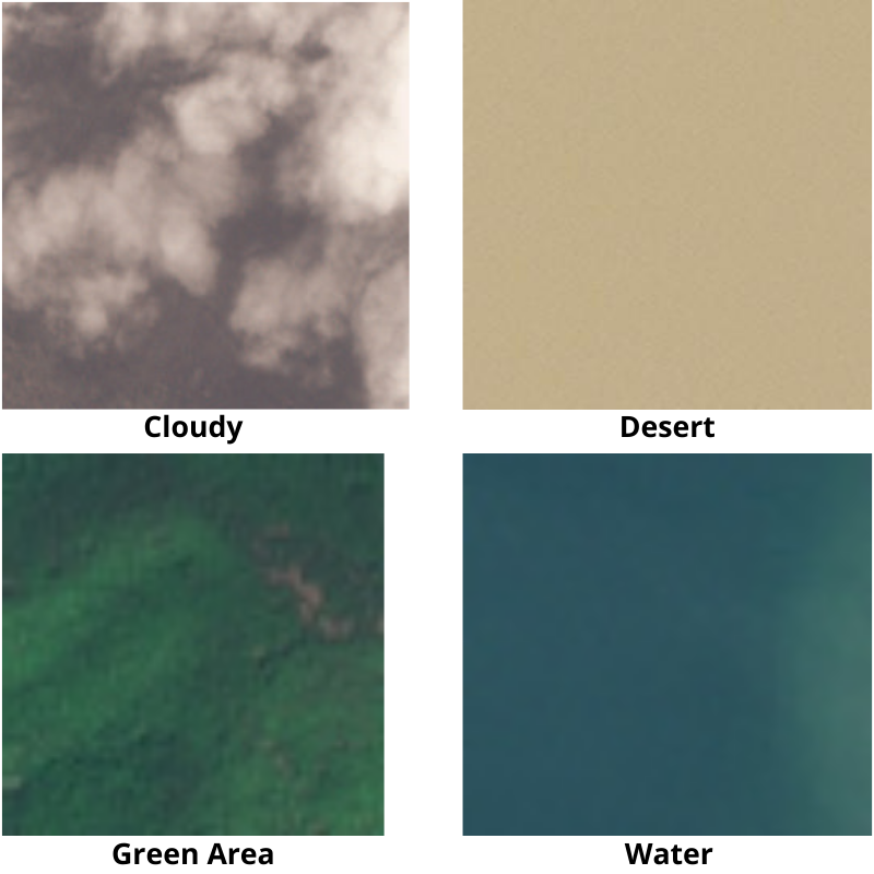
One thing to note here is that the desert and cloudy class images are colored images of 256×256 dimensions which is more than fine if resizing is required. But the green_area and water class images are only 64×64 dimensional images, they are colored images too. But if increasing their image size when augmenting them, their features may not be as clear as the other two classes. This can cause some problems in training these two classes. We will look into it later on.

If you want to explore the dataset a bit more, be sure to do that before moving on to the next section. Also, be sure to download the data before moving ahead. We will see how to structure it in the next section.

Directory Structure

Let’s take a look at the directory structure for this project.

├── input
│   ├── data
│   │   ├── cloudy [1500 entries exceeds filelimit, not opening dir]
│   │   ├── desert [1131 entries exceeds filelimit, not opening dir]
│   │   ├── green_area [1500 entries exceeds filelimit, not opening dir]
│   │   └── water [1500 entries exceeds filelimit, not opening dir]
│   └── test_data
│       ├── cloudy.jpeg
│       ├── desert.jpeg
│       ├── green_area.jpeg
│       └── water.jpeg
├── outputs
│   ├── accuracy.png
│   ├── cloudy.png
│   ├── desert.png
│   ├── forest_area.png
│   ├── green_area.png
│   ├── loss.png
│   ├── model.pth
│   └── water.png
├── datasets.py
├── inference.py
├── model.py
├── train.py
└── utils.py

In the parent project directory we have:

• The input directory which holds the data subdirectory and which in turn contains the dataset class folders. It will be easiest for you to follow along if you keep your directory structure similar. That way you do not need to change anything in the Python code files. The test_data subdirectory contains the images from internet which we will use for inference after training the model. These are completely new images and unseen by the trained PyTorch ResNet34 model.
• The outputs directory contains the images, plots, and trained model that are training and inference pipeline will genetate.
• 5 Python files. We will get into the details of these later on.

If you download the zipped code file for this tutorial, then you will already have everything in place. You just need to download the dataset from Kaggle and properly place it. In fact, you will also have access to the trained model which you can directly use for inference. But for most learning, I recommend that you retrain the model while following the tutorial.

PyTorch Version

This code has been run and tested with PyTorch version 1.9.0. But it should run fine from version 1.7.0 till version 1.9.0. Feel free to install the latest version from here.

Satellite Image Classification using PyTorch ResNet34

We will start the coding part of this tutorial/mini-project from here.

There are five Python files. We will tackle them in the following order:

• utils.py
• datasets.py
• model.py
• train.py
• inference.py – after training completes and we have the PyTorch ResNet34 trained model.

Many of the code such as the utility and helper functions, the training and validation functions, will be similar to my previous PyTorch image classification posts. For that reason, we may not dive too deep into their explanation. If you have been coding in PyTorch for some time now, these should be pretty easy to follow along.

Utility and Helper Functions

We have two helper functions, one to save the trained model, and the other one to save the loss and accuracy graphs.

These functions will go into the utils.py file.

The following code block contains the import statements and the save_model() function.

import torch
import matplotlib
import matplotlib.pyplot as plt

matplotlib.style.use('ggplot')


def save_model(epochs, model, optimizer, criterion):
    """
    Function to save the trained model to disk.
    """
    torch.save({
                'epoch': epochs,
                'model_state_dict': model.state_dict(),
                'optimizer_state_dict': optimizer.state_dict(),
                'loss': criterion,
                }, 'outputs/model.pth')

We are saving the number of epochs trained for, the model state dictionary, the optimizer state dictionary, and even the loss function in model.pth. This extra information becomes very helpful when trying to resume training later on.

Next, we have the function to save the loss and accuracy graphs.

def save_plots(train_acc, valid_acc, train_loss, valid_loss):
    """
    Function to save the loss and accuracy plots to disk.
    """
    # accuracy plots
    plt.figure(figsize=(10, 7))
    plt.plot(
        train_acc, color='green', linestyle='-', 
        label='train accuracy'
    )
    plt.plot(
        valid_acc, color='blue', linestyle='-', 
        label='validataion accuracy'
    )
    plt.xlabel('Epochs')
    plt.ylabel('Accuracy')
    plt.legend()
    plt.savefig('outputs/accuracy.png')
    
    # loss plots
    plt.figure(figsize=(10, 7))
    plt.plot(
        train_loss, color='orange', linestyle='-', 
        label='train loss'
    )
    plt.plot(
        valid_loss, color='red', linestyle='-', 
        label='validataion loss'
    )
    plt.xlabel('Epochs')
    plt.ylabel('Loss')
    plt.legend()
    plt.savefig('outputs/loss.png')

The save_plots() function accepts the respective loss and accuracy lists for training and validation. The graphs are saved in the outputs folder.

For now, these two helper functions are enough for our needs.

Preparing the Dataset

Preparing the dataset is also going to be pretty easy as PyTorch provides many functionalities.

While preparing the dataset, we will write the code in the datasets.py file.

Let’s import the required PyTorch modules and define a few constants.

import torch

from torch.utils.data import DataLoader, Subset
from torchvision import datasets, transforms

# ratio of data to use for validation
valid_split = 0.2
# batch size
batch_size = 64
# path to the data root directory
root_dir = 'input/data'

As we can see, we will use 20% of the data for validation. The batch size is 64. If you are training on your local machine and face OOM (Out Of Memory) issues for GPU, then consider lowering the batch size, maybe to 32 or 16.

The Training and Validation Transforms

The next code block contains the training and validation transform.

# define the training transforms and augmentations
train_transform = transforms.Compose([
    transforms.Resize(224),
    transforms.RandomHorizontalFlip(p=0.5),
    transforms.RandomVerticalFlip(p=0.5),
    transforms.GaussianBlur(kernel_size=(5, 9), sigma=(0.1, 5)),
    transforms.RandomRotation(degrees=(30, 70)),
    transforms.ToTensor(),
    transforms.Normalize(
        mean=[0.485, 0.456, 0.406],
        std=[0.229, 0.224, 0.225]
    )
])

valid_transform = transforms.Compose([
    transforms.Resize((224, 224)),
    transforms.ToTensor(),
    transforms.Normalize(
        mean=[0.485, 0.456, 0.406],
        std=[0.229, 0.224, 0.225]
    )
])

For training, along with the transforms, we are also augmenting the images to prevent overfitting. Without augmentations, the training accuracy hit above 99% pretty quickly while the validation accuracy was still quite low. So, these augmentations are mostly from experimentations, and what worked best for this dataset.

Also, you can see that we are applying the ImageNet stats for the normalization. This is because we will be using a pretrained ResNet34 model.

For the validation, we are resizing the images, converting them to tensors, and normalizing them.

The Data Loaders

# initial entire and test datasets
dataset = datasets.ImageFolder(root_dir, transform=train_transform)
dataset_test = datasets.ImageFolder(root_dir, transform=valid_transform)

print(f"Classes: {dataset.classes}")

dataset_size = len(dataset)
print(f"Total number of images: {dataset_size}")

valid_size = int(valid_split*dataset_size)

# training and validation sets
indices = torch.randperm(len(dataset)).tolist()
dataset_train = Subset(dataset, indices[:-valid_size])
dataset_valid = Subset(dataset_test, indices[-valid_size:])

print(f"Total training images: {len(dataset_train)}")
print(f"Total valid_images: {len(dataset_valid)}")

# training and validation data loaders
train_loader = DataLoader(
    dataset_train, batch_size=batch_size, shuffle=True, num_workers=4
)
valid_loader = DataLoader(
    dataset_valid, batch_size=batch_size, shuffle=False, num_workers=4
)

Let’s focus on what is going on in the above code block.

• First of all, we can see that we are defining dataset and dataset_test by using the ImageFolder class on the entire directory. This means that currently both of them hold the exact same dataset but with different transforms. There is a reason for this.
• On line 43, we are defining valid_size which gives us the number of images we want for the validation set.
• On line 46, the indices list holds all the indices for the entire dataset length.
• Out of these, we use everything before valid_size for dataset_train from dataset and the rest for dataset_valid from dataset_test. This gives us the proper training and validation dataset.
• Then from line 54, we define the training and validation dataloaders.

If you are using Windows OS, then the num_workers=4 may give a BrokenPipe error. For that, you can use num_workers=0.

This completes the preparation of our Satellite Image dataset.

The PyTorch ResNet34 Neural Network Model

As discussed before we will use the PyTorch ResNet34 model for satellite image classification.

PyTorch already provides the ImageNet pretrained model for ResNet34. We just have to change the final layer with the correct number of classes.

Let’s write the model preparation code in model.py file.

import torchvision.models as models
import torch.nn as nn

def build_model(pretrained=True, fine_tune=True, num_classes=1):
    if pretrained:
        print('[INFO]: Loading pre-trained weights')
    elif not pretrained:
        print('[INFO]: Not loading pre-trained weights')
    model = models.resnet34(pretrained=pretrained)

    if fine_tune:
        print('[INFO]: Fine-tuning all layers...')
        for params in model.parameters():
            params.requires_grad = True
    elif not fine_tune:
        print('[INFO]: Freezing hidden layers...')
        for params in model.parameters():
            params.requires_grad = False
            
    # change the final classification head, it is trainable
    model.fc = nn.Linear(512, num_classes)
    return model

Through the parameters to the build_model() function, we are controlling:

• Whether we want the pretrained model or not.
• Whether we want to fine_tune the intermediate layers.
• And the number of classes, that is num_classes.

We are changing the final layer of the model on line 21.

The Training Script

We have the helper functions, model, and dataset ready by now.

The final step before training would be to write the training script.

Let’s do that in the train.py Python script. This will be an executable Python file.

import torch
import argparse
import torch.nn as nn
import torch.optim as optim

from model import build_model
from utils import save_model, save_plots
from datasets import train_loader, valid_loader, dataset
from tqdm.auto import tqdm

# construct the argument parser
parser = argparse.ArgumentParser()
parser.add_argument('-e', '--epochs', type=int, default=20,
    help='number of epochs to train our network for')
args = vars(parser.parse_args())

The above code block imports all the library modules and the ones we have written till now. Along with that, we also have the argument parser which controls the number of epochs we want the model to train for using the --epochs flag.

The Learning Parameters, the Model, Optimizer and Loss Function

The next code block defines the learning rate, computation device, the number of epochs from the argument parser flag. We also build the ResNet34 model and define the optimizer and loss function.

# learning_parameters 
lr = 0.001
epochs = args['epochs']
device = ('cuda' if torch.cuda.is_available() else 'cpu')
print(f"Computation device: {device}\n")


# build the model
model = build_model(
    pretrained=True, fine_tune=False, num_classes=len(dataset.classes)
).to(device)
# total parameters and trainable parameters
total_params = sum(p.numel() for p in model.parameters())
print(f"{total_params:,} total parameters.")
total_trainable_params = sum(
    p.numel() for p in model.parameters() if p.requires_grad)
print(f"{total_trainable_params:,} training parameters.\n")

# optimizer
optimizer = optim.Adam(model.parameters(), lr=lr)
# loss function
criterion = nn.CrossEntropyLoss()

We are calling the build_model() function with:

• pretrained=True
• fine_tune=False
• num_classes=len(dataset.classes)

That will give us the desired model we want to train.

The optimizer is Adam with a learning rate of 0.001, and the loss function is Cross Entropy.

The Training and Validation Functions

The training function will be a standard image classification training function in PyTorch. We do the forward pass, calculate the losses, backpropagate the gradients, and update the parameters.

# training
def train(model, trainloader, optimizer, criterion):
    model.train()
    print('Training')
    train_running_loss = 0.0
    train_running_correct = 0
    counter = 0
    for i, data in tqdm(enumerate(trainloader), total=len(trainloader)):
        counter += 1
        image, labels = data
        image = image.to(device)
        labels = labels.to(device)
        optimizer.zero_grad()
        # forward pass
        outputs = model(image)
        # calculate the loss
        loss = criterion(outputs, labels)
        train_running_loss += loss.item()
        # calculate the accuracy
        _, preds = torch.max(outputs.data, 1)
        train_running_correct += (preds == labels).sum().item()
        # backpropagation
        loss.backward()
        # update the optimizer parameters
        optimizer.step()
    
    # loss and accuracy for the complete epoch
    epoch_loss = train_running_loss / counter
    epoch_acc = 100. * (train_running_correct / len(trainloader.dataset))
    return epoch_loss, epoch_acc

After each epoch, the function returns the loss and accuracy for that epoch.

Next, the validation function. It is going to be slightly different apart from the obvious no backpropagation, and no parameter updates.

# validation
def validate(model, testloader, criterion, class_names):
    model.eval()
    print('Validation')
    valid_running_loss = 0.0
    valid_running_correct = 0
    counter = 0
    
    # we need two lists to keep track of class-wise accuracy
    class_correct = list(0. for i in range(len(class_names)))
    class_total = list(0. for i in range(len(class_names)))
    
    with torch.no_grad():
        for i, data in tqdm(enumerate(testloader), total=len(testloader)):
            counter += 1
            
            image, labels = data
            image = image.to(device)
            labels = labels.to(device)
            # forward pass
            outputs = model(image)
            # calculate the loss
            loss = criterion(outputs, labels)
            valid_running_loss += loss.item()
            # calculate the accuracy
            _, preds = torch.max(outputs.data, 1)
            valid_running_correct += (preds == labels).sum().item()
            
            # calculate the accuracy for each class
            correct  = (preds == labels).squeeze()
            for i in range(len(preds)):
                label = labels[i]
                class_correct[label] += correct[i].item()
                class_total[label] += 1
        
    # loss and accuracy for the complete epoch
    epoch_loss = valid_running_loss / counter
    epoch_acc = 100. * (valid_running_correct / len(testloader.dataset))
    
    # print the accuracy for each class after every epoch
    print('\n')
    for i in range(len(class_names)):
        print(f"Accuracy of class {class_names[i]}: {100*class_correct[i]/class_total[i]}")
    print('\n')
        
    return epoch_loss, epoch_acc

On lines 77 and 78, we have two lists, class_total and class_correct. We need these two lists to keep track of the class wise accuracy. Now, if you see from lines 97 to 101 is where we calculate the accuracy for each individual class. And we print those accuracies on lines 109 and 110.

Now, why class-wise accuracy? Previously, we had seen that the water and green_area class images are smaller than the other two classes. There is a very high chance that the model will not be learning the features of these classes as well as the other ones. Therefore, to validate our doubt, we have these class wise accuracies as well. Even if the model learns well, we have extra information about each of the classes, which is anyways good.

The Training Loop

Finally, the training loop.

# lists to keep track of losses and accuracies
train_loss, valid_loss = [], []
train_acc, valid_acc = [], []
# start the training
for epoch in range(epochs):
    print(f"[INFO]: Epoch {epoch+1} of {epochs}")
    train_epoch_loss, train_epoch_acc = train(model, train_loader, 
                                              optimizer, criterion)
    valid_epoch_loss, valid_epoch_acc = validate(model, valid_loader,  
                                                 criterion, dataset.classes)
    train_loss.append(train_epoch_loss)
    valid_loss.append(valid_epoch_loss)
    train_acc.append(train_epoch_acc)
    valid_acc.append(valid_epoch_acc)
    print(f"Training loss: {train_epoch_loss:.3f}, training acc: {train_epoch_acc:.3f}")
    print(f"Validation loss: {valid_epoch_loss:.3f}, validation acc: {valid_epoch_acc:.3f}")
    print('-'*50)

# save the trained model weights
save_model(epochs, model, optimizer, criterion)
# save the loss and accuracy plots
save_plots(train_acc, valid_acc, train_loss, valid_loss)
print('TRAINING COMPLETE')

On lines 115 and 116, we initialize four lists to store the loss and accuracy values for training and validation epochs as the training goes on.

After each epoch, we print the training and validation accuracy as well as the loss value.

On lines 133 and 135, we save the trained model and the graphs.

This completes all the code we need for training.

Execute train.py To Start Training

Open your command line/terminal in the directory where the Python files are present and execute the following command.

python train.py --epochs 100 

We are training for 100 epochs and the following block shows the truncated output.

Classes: ['cloudy', 'desert', 'green_area', 'water']
Total number of images: 5631
Total training images: 4505
Total valid_images: 1126
Computation device: cuda

[INFO]: Loading pre-trained weights
Downloading: "https://download.pytorch.org/models/resnet34-333f7ec4.pth" to /root/.cache/torch/hub/checkpoints/resnet34-333f7ec4.pth
100%|██████████████████████████████████████| 83.3M/83.3M [00:04<00:00, 18.9MB/s]
[INFO]: Freezing hidden layers...
21,286,724 total parameters.
2,052 training parameters.

[INFO]: Epoch 1 of 100
Training
100%|███████████████████████████████████████████| 71/71 [00:38<00:00,  1.84it/s]
Validation
100%|███████████████████████████████████████████| 18/18 [00:04<00:00,  4.36it/s]


Accuracy of class cloudy: 76.84887459807074
Accuracy of class desert: 67.71300448430493
Accuracy of class green_area: 89.43661971830986
Accuracy of class water: 96.42857142857143


Training loss: 0.518, training acc: 86.637
Validation loss: 0.614, validation acc: 83.570
--------------------------------------------------
Training loss: 0.028, training acc: 98.935
Validation loss: 0.144, validation acc: 95.560
--------------------------------------------------
[INFO]: Epoch 100 of 100
Training
100%|███████████████████████████████████████████| 71/71 [00:35<00:00,  1.97it/s]
Validation
100%|███████████████████████████████████████████| 18/18 [00:03<00:00,  5.44it/s]


Accuracy of class cloudy: 99.03536977491962
Accuracy of class desert: 96.8609865470852
Accuracy of class green_area: 89.43661971830986
Accuracy of class water: 94.48051948051948


Training loss: 0.035, training acc: 98.713
Validation loss: 0.165, validation acc: 94.938
--------------------------------------------------
TRAINING COMPLETE

As you can see in the above block, after each epoch, the class-wise accuracy gets printed. We need to keep in mind that this is the validation accuracy. And as expected, by the end of 100 epochs, the green_area and water classes have less accuracy than the other two classes.

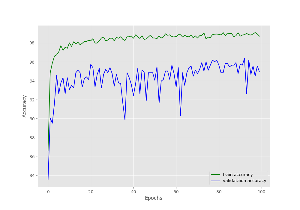
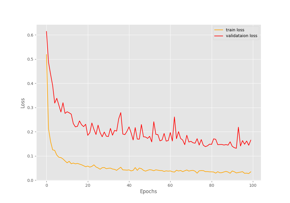
Both the accuracy and loss graphs seem to fluctuate quite a bit. But they seem to keep on improving as well. Some regularization techniques would surely help here.

Now, let’s write the script for carrying out inference.

The Inference Script

The inference script will be quite straightforward as well.

We will write the code in inference.py Python script.

Starting with the imports, the argument parser, and the computation device.

import torch
import cv2
import torchvision.transforms as transforms
import argparse

from model import build_model

# construct the argument parser
parser = argparse.ArgumentParser()
parser.add_argument('-i', '--input', 
    default='input/test_data/cloudy.jpeg',
    help='path to the input image')
args = vars(parser.parse_args())

# the computation device
device = 'cpu'

All the inference will happen on the CPU. For image classification inference, using a GPU device is not mandatory at all, a CPU will do just fine.

Loading the Trained Model and Preprocessing Transforms

The next code block defines the class names, loads the trained model, and defines the preprocessing transforms as well.

# list containing all the labels
labels = ['cloudy', 'desert', 'green_area', 'water']

# initialize the model and load the trained weights
model = build_model(
    pretrained=False, fine_tune=False, num_classes=4
).to(device)
print('[INFO]: Loading custom-trained weights...')
checkpoint = torch.load('outputs/model.pth', map_location=device)
model.load_state_dict(checkpoint['model_state_dict'])
model.eval()

# define preprocess transforms
transform = transforms.Compose([
    transforms.ToPILImage(),
    transforms.Resize(224),
    transforms.ToTensor(),
    transforms.Normalize(
        mean=[0.485, 0.456, 0.406],
        std=[0.229, 0.224, 0.225]
    )
]) 

For the preprocessing, we just need to convert the image into PIL image format, resize it, convert it to tensor, and apply the normalization.

Reading the Image and the Forward Pass

Let’s read the image and pass the image through the model.

# read and preprocess the image
image = cv2.imread(args['input'])
# get the ground truth class
gt_class = args['input'].split('/')[-1].split('.')[0]
orig_image = image.copy()
# convert to RGB format
image = cv2.cvtColor(image, cv2.COLOR_BGR2RGB)
image = transform(image)
# add batch dimension
image = torch.unsqueeze(image, 0)
with torch.no_grad():
    outputs = model(image.to(device))
output_label = torch.topk(outputs, 1)
pred_class = labels[int(output_label.indices)]
cv2.putText(orig_image, 
    f"GT: {gt_class}",
    (10, 25),
    cv2.FONT_HERSHEY_SIMPLEX, 
    1, (0, 255, 0), 2, cv2.LINE_AA
)
cv2.putText(orig_image, 
    f"Pred: {pred_class}",
    (10, 55),
    cv2.FONT_HERSHEY_SIMPLEX, 
    1, (0, 0, 255), 2, cv2.LINE_AA
)
print(f"GT: {gt_class}, pred: {pred_class}")
cv2.imshow('Result', orig_image)
cv2.waitKey(0)
cv2.imwrite(f"outputs/{gt_class}.png",
    orig_image)

After reading the image, we are getting the ground truth label on line 42. All the test images have a name in the format <ground_truth_class_name>.jpeg so that we can easily extract the information without any other dependency.

After the required preprocessing, the forward pass happens on line 50 and we extract the predicted class name on line 52, which is pred_class.

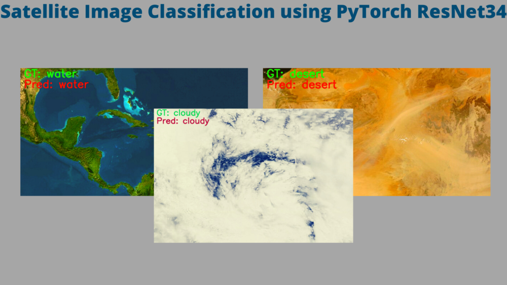
Starting from line 53, we put the ground truth class name and the predicted class on the original image, show the output on the screen, and save it to disk as well.

Executing the Inference Script

We have four test images, in the input/test_data directory. Let’s run them one by one and check out the results.

python inference.py --input input/test_data/cloudy.jpeg

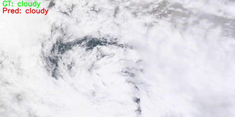
That’s great. The trained PyTorch ResNet34 model is able to correctly predict the class as cloudy.

Moving on to the next test image.

python inference.py --input input/test_data/desert.jpeg

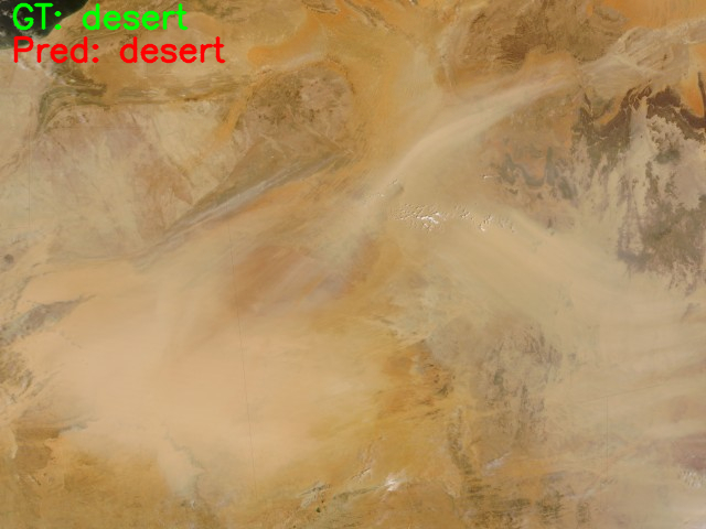
This time also the prediction is correct.

Now, for the green_area image.

python inference.py --input input/test_data/green_area.jpeg

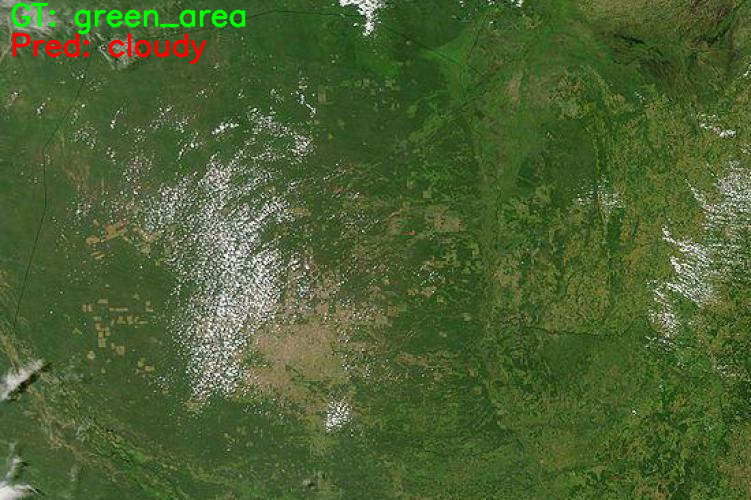
Here, the model is making mistake. It is predicting the image as cloudy class. If you remember, the model struggled the most with the green_area class while training. That seems to reflect during inference as well.

Only one more image is left.

python inference.py --input input/test_data/water.jpeg

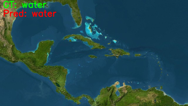
This prediction is correct. So, it seems that the model is only struggling with the green_area class.

Takeaways and Further Approaches

We can improve the training and inference quite a bit.

• Training for longer should surely help.
• If the model will overfit, we can apply other regularization techniques like dropout before the final layer and applying learning rate scheduler.
• Collecting more images for training should help as well.
• And we should also try other pre-trained models, or even training from scratch just for experimentation.

If you try any of the above pointers, you may report your findings in the comment section for others to know.

Summary and Conclusion

In this tutorial, we tried a small image classification project. We tried satellite image classification using the PyTorch ResNet34 model. We also carried out inference on new images and discussed how to further improve the project. I hope that you find this post useful.

If you have any doubts, thoughts, or suggestions, please leave them in the comment section. I will surely address them.

You can contact me using the Contact section. You can also find me on LinkedIn, and Twitter.

Credits and attributions for inference images:

• cloudy.jpeg: https://blog.mapbox.com/cloudy-satellite-imagery-a-chronicle-of-imagery-collection-over-nepal-post-disaster-8830e3cbd1f.
• desert.jpeg: https://earthobservatory.nasa.gov/images/19845/saharan-dust-storm.
• green_area: https://www.un-spider.org/news-and-events/news/fao-and-norway-help-developing-countries-monitor-their-forest-through-earth.
• water.jpeg: http://wallpaperweb.org/wallpaper/space/caribbean-sea_59884.htm.