Saving and Loading the Best Model in PyTorch

Often while training deep learning models, we tend to save and use the latest checkpoint for inference. While in most cases, it may not matter much, but there is a high chance that we are using an overfit model. It is always a better idea to use the best model for inference or testing on images and videos after training. In this tutorial, you will learn about easily saving and loading the best model in PyTorch.

A Bit of Background…

Using the last model checkpoint or state dictionary to load the weights might prove to be a bit harmful. The model might be an overfit one. If the test data is from the same sample space as the training data, then the results might even be good. But the real problem will arise when we try to run inference on a similar type of data but completely unseen by the model. In those cases, there is a chance that the model will perform worse.

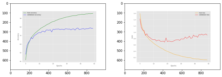
For example, in the above graphs, although we can see the accuracies improving till the end, the validation loss is deteriorating. This means that the model is overfitting after a certain set of epochs. There are regularization methods to avoid this. But what if we want to use a set of weights from this training? Obviously, the last epoch weights are the overfit ones. So, we need the weights from the best performing epoch. But how to save the best weights in PyTorch while training a deep learning model? That is exactly what we will be trying to learn in this tutorial.

Let’s check out the points that we will cover in this tutorial.

• We will train a deep learning model on the CIFAR10 dataset.
• It is going to be the ResNet18 model.
• We will use minimal regularization techniques while training to ensure that the model overfits. So, we will need to save the best weights and not the last epochs weights for inferencing.
• We will also train for a bit longer than required so that the last epoch’s weights are not the best, rather they are overfit ones.
• After the training and saving the best model, we will carry out testing to see that the best weights are actually giving the better results when compare to the overfit ones in PyTorch.

The CIFAR10 Dataset

The CIFAR10 dataset is a very well know image classification dataset in the deep learning and computer vision community. There is a very high chance that you are already familiar with the dataset. Still, let’s go over some of the important aspects of it.

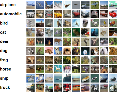
The CIFAR10 dataset contains 60000 images spanning over 10 classes such as:

• airplane
• automobile
• bird
• cat
• deer
• dog
• frog
• horse
• sheep
• truck

Out of the 60000 images, 50000 images are for training and the rest 10000 are for testing. All the images are 32×32 RGB images.

Although it is a fairly old dataset, still achieving very high accuracy on the CIFAR10 dataset can be challenging, especially for beginners.

While we will not focus on achieving any state-of-the-art result in this tutorial, we will try our best to get a test accuracy of more than 75%. That too with the best possible non-overfit model. It should be a good challenge for us. Also, we can easily load the CIFAR10 dataset using torchvision.datasets in PyTorch.

Project Directory Structure

For saving the best model in the PyTorch project, we will use the following directory structure.

│   datasets.py
│   model.py
│   test.py
│   train.py
│   utils.py
│   
├───data
│   │   cifar-10-python.tar.gz
│   │   
│   └───cifar-10-batches-py
│           batches.meta
│           ...
│           
├───outputs
│       accuracy.png
│       best_model.pth
│       final_model.pth
│       loss.png

• As we can see, we have five Python files that we will use in this project. We will get into the details of these later on.
• The data directory gets generated automatically when downloading the CIFAR10 dataset using PyTorch for the first time. The internal contents will be downloaded automatically as well.
• The outputs folder contains the weights while saving the best and last epoch models in PyTorch during training. It also contains the loss and accuracy graphs.

If you download the zipped files for this tutorial, you will have all the directories in place. You can follow along easily and run the training and testing scripts without any delay.

The PyTorch Version

All the code in this tutorial has been written and tested with PyTorch 1.9.1 (the latest at the time of writing this). As this tutorial does not use any fancy features, optimizers, or activation functions, you should be good to follow along even with a slightly older version. If you face any issues, consider installing the latest version at the time of your reading.

Saving and Loading the Best Model in PyTorch

The coding part of this project is going to be very similar to the PyTorch image classification one. The only differences are:

• Code for saving the best model.
• Testing the best epoch saved model and the last epoch saved model on a test set.

Before we can begin the training, we have four Python files to write code for.

Utility Classes and Functions

We will begin with a few utility classes and helper functions. This is where we will write the class to save the best model as well.

All this code will go into the utils.py file.

Let’s begin by writing a Python class that will save the best model while training.

import torch
import matplotlib.pyplot as plt

plt.style.use('ggplot')

class SaveBestModel:
    """
    Class to save the best model while training. If the current epoch's 
    validation loss is less than the previous least less, then save the
    model state.
    """
    def __init__(
        self, best_valid_loss=float('inf')
    ):
        self.best_valid_loss = best_valid_loss
        
    def __call__(
        self, current_valid_loss, 
        epoch, model, optimizer, criterion
    ):
        if current_valid_loss < self.best_valid_loss:
            self.best_valid_loss = current_valid_loss
            print(f"\nBest validation loss: {self.best_valid_loss}")
            print(f"\nSaving best model for epoch: {epoch+1}\n")
            torch.save({
                'epoch': epoch+1,
                'model_state_dict': model.state_dict(),
                'optimizer_state_dict': optimizer.state_dict(),
                'loss': criterion,
                }, 'outputs/best_model.pth')

The above is a very simple class to save the best model while the training goes on. There are to few points to note here:

• The __init__() method first initializes the self.best_valid_loss with infinity value when we create an instance of the class. This is to ensure that any loss from the model will be less than the initial value.
• After creating the instance of the class, we just need to call that instance and the __call__() method will be executed. This means that we need to pass the current epoch’s validation loss, the current epoch number, the model instance, the optimizer, and the loss function as well.

If the current epoch’s loss is less than the last best validation loss, then we update self.best_valid_loss. After that, we save the model’s state dictionary along with the epoch number.

The above is a very simple class and of course, there are other ways to achieve what we are trying to achieve here. For now, let’s keep things simple.

Function to Save the Last Epoch’s Model and the Loss & Accuracy Graphs

The next block contains the code to save the model after the training completes, that is, the last epoch’s model.

def save_model(epochs, model, optimizer, criterion):
    """
    Function to save the trained model to disk.
    """
    print(f"Saving final model...")
    torch.save({
                'epoch': epochs,
                'model_state_dict': model.state_dict(),
                'optimizer_state_dict': optimizer.state_dict(),
                'loss': criterion,
                }, 'outputs/final_model.pth')

We will call this function after the training iterations for all the epochs are complete.

The final helper function is for saving the loss and accuracy graphs for training and validation.

def save_plots(train_acc, valid_acc, train_loss, valid_loss):
    """
    Function to save the loss and accuracy plots to disk.
    """
    # accuracy plots
    plt.figure(figsize=(10, 7))
    plt.plot(
        train_acc, color='green', linestyle='-', 
        label='train accuracy'
    )
    plt.plot(
        valid_acc, color='blue', linestyle='-', 
        label='validataion accuracy'
    )
    plt.xlabel('Epochs')
    plt.ylabel('Accuracy')
    plt.legend()
    plt.savefig('outputs/accuracy.png')
    
    # loss plots
    plt.figure(figsize=(10, 7))
    plt.plot(
        train_loss, color='orange', linestyle='-', 
        label='train loss'
    )
    plt.plot(
        valid_loss, color='red', linestyle='-', 
        label='validataion loss'
    )
    plt.xlabel('Epochs')
    plt.ylabel('Loss')
    plt.legend()
    plt.savefig('outputs/loss.png')

That’s it for the utils.py file. Next, let’s prepare the CIFAR10 dataset.

Prepare the CIFAR10 Dataset

The code to prepare the CIFAR10 dataset for this tutorial is going to be a bit longer than usual. We need one training set, one validation set, and one test set as well. We will use the test set after the training completes. And creating these three sets instead of the general training and validation will take a few extra lines of code.

This code will go into the datasets.py file.

Beginning with the imports and a few constants we need along the way.

import torch
import torchvision
import torchvision.transforms as transforms

from torch.utils.data import DataLoader, Subset

# data constants
BATCH_SIZE = 64
VALID_SPLIT = 0.2
NUM_WORKERS = 0

The above code block defines the constants for the:

• Batch size for the CIFAR10 dataset.
• The split for the validation set, that is 20%.
• And the number of sub process workers. Let’s keep these to 0 for now.

The Training and Validation Transforms

For training, we will use horizontal and vertical flip augmentations along with the preprocessing transforms. The validation transforms consist only of the preprocessing steps.

# transforms and augmentations for training
train_transform = transforms.Compose([
    transforms.RandomHorizontalFlip(p=0.5),
    transforms.RandomVerticalFlip(p=0.5),
    transforms.ToTensor(),
    transforms.Normalize((0.5, 0.5, 0.5), (0.5, 0.5, 0.5))
])

# transforms for validation and testing
valid_transform = transforms.Compose([
    transforms.ToTensor(),
    transforms.Normalize((0.5, 0.5, 0.5), (0.5, 0.5, 0.5))
])

The flip augmentations are applied with a probability of 0.5. And the valid_transform will also be applied to the test dataset.

Function to Create the Dataset

The next function, that is  create_datasets() will create and return the train, validation, and test dataset.

# function to create the datasets
def create_datasets():
    """
    Function to build the training, validation, and testing dataset.
    """
    # we choose the `train_dataset` and `valid_dataset` from the same...
    # ... distribution and later one divide 
    train_dataset = torchvision.datasets.CIFAR10(root='./data', train=True,
                                            download=True, transform=train_transform)
    valid_dataset = torchvision.datasets.CIFAR10(root='./data', train=True,
                                            download=True, transform=valid_transform)
    # this is the final test dataset to be used after training and validation completes
    dataset_test = torchvision.datasets.CIFAR10(root='./data', train=False,
                                       download=True, transform=valid_transform)

    # get the training dataset size, need this to calculate the...
    # number if validation images   
    train_dataset_size = len(train_dataset)
    # validation size = number of validation images
    valid_size = int(VALID_SPLIT*train_dataset_size)

    # all the indices from the training set
    indices = torch.randperm(len(train_dataset)).tolist()
    # final train dataset discarding the indices belonging to `valid_size` and after
    dataset_train = Subset(train_dataset, indices[:-valid_size])
    # final valid dataset from indices belonging to `valid_size` and after
    dataset_valid = Subset(valid_dataset, indices[-valid_size:])
    print(f"Total training images: {len(dataset_train)}")
    print(f"Total validation images: {len(dataset_valid)}")
    print(f"Total test images: {len(dataset_test)}")
    return dataset_train, dataset_valid, dataset_test

If you take a look at lines 32 and 34, then we are getting the train_dataset and valid_dataset from the same training distribution of CIFAR10. We are doing this so that we can apply different sets of transforms to both. To create the final training and validation datasets, we are getting the valid_size from the VALID_SPLIT and then indices stores all the indices from the training set. The dataset_train (final training set) contains all the images from train_dataset before valid_size. And dataset_valid (final validation set) contains all the images from valid_dataset after the valid_size number of indices.

The dataset_test is from the validation distribution and we will use this to create the test data loader which will be used for testing at the end.

Doing the above, we are able to get three different splits and apply the required augmentations to the training set as well.

Function to Create the Data Loaders

The final function for the dataset preparation is creating the three data loaders.

def create_data_loaders(dataset_train, dataset_valid, dataset_test):
    """
    Function to build the data loaders.

    Parameters:
    :param dataset_train: The training dataset.
    :param dataset_valid: The validation dataset.
    :param dataset_test: The test dataset.
    """
    train_loader = DataLoader(
        dataset_train, batch_size=BATCH_SIZE, shuffle=True, num_workers=NUM_WORKERS
    )
    valid_loader = DataLoader(
        dataset_valid, batch_size=BATCH_SIZE, shuffle=False, num_workers=NUM_WORKERS
    )
    test_loader = DataLoader(
        dataset_test, batch_size=BATCH_SIZE, shuffle=False, num_workers=NUM_WORKERS
    )
    return train_loader, valid_loader, test_loader

The create_data_loaders() accepts the three dataset splits as parameters and returns the respective data loaders.

This completes the dataset preparation part as well. We will call the functions we need from this module as we start training our neural network.

The Neural Network Model

For saving the best model in PyTorch for any dataset, the neural network architecture plays a crucial role.

Here, instead of writing a custom neural network model, we use the ResNet18 model from torchvision.models.

Let’s check out the code to prepare the neural network in PyTorch. We will write this code in the model.py file.

import torchvision.models as models
import torch.nn as nn

def build_model(pretrained=True, fine_tune=True, num_classes=1):
    """
    Function to build the neural network model. Returns the final model.

    Parameters
    :param pretrained (bool): Whether to load the pre-trained weights or not.
    :param fine_tune (bool): Whether to train the hidden layers or not.
    :param num_classes (int): Number of classes in the dataset. 
    """
    if pretrained:
        print('[INFO]: Loading pre-trained weights')
    elif not pretrained:
        print('[INFO]: Not loading pre-trained weights')
    model = models.resnet18(pretrained=pretrained)

    if fine_tune:
        print('[INFO]: Fine-tuning all layers...')
        for params in model.parameters():
            params.requires_grad = True
    elif not fine_tune:
        print('[INFO]: Freezing hidden layers...')
        for params in model.parameters():
            params.requires_grad = False
            
    # change the final classification head, it is trainable
    model.fc = nn.Linear(512, num_classes)
    return model

In the above code block, the docstring provides the information about all the parameters that the build_model() function accepts.

While building the PyTorch ResNet18 model, we will not load any ImageNet pre-trained weights. Also, we will train all the hidden layers. For the number of classes, we are modifying the final fully connected layer on line 29. For the CIFAR10 dataset, this is going to be 10.

The Training Script

Now, we are down to the training script. This is the Python file that we will run from the command line to train and validate our network for the required number of epochs.

All the code here will go into the train.py script.

This will contain a very standard set of image classification code using PyTorch. Although most of the things are self-explanatory, we will go over a few of the important bits of code.

Starting with the import statements and the construction of the argument parser.

import torch
import argparse
import torch.nn as nn
import torch.optim as optim

from tqdm.auto import tqdm

from model import build_model
from datasets import create_datasets, create_data_loaders
from utils import save_model, save_plots, SaveBestModel

# construct the argument parser
parser = argparse.ArgumentParser()
parser.add_argument('-e', '--epochs', type=int, default=20,
    help='number of epochs to train our network for')
args = vars(parser.parse_args())

We are importing all the required classes and functions from our own modules. This contains the SaveBestModel class as well.

For the argument parser, we just have the --epochs flag. This is to provide the number of epochs from the command line argument we want to train for.

Prepare the Required Data Loaders and Define the Learning Parameters

For the training script, we just need the training and validation data loaders. We will use the test data loader while testing the model after training.

# get the training, validation and test_datasets
train_dataset, valid_dataset, test_dataset = create_datasets()
# get the training and validaion data loaders
train_loader, valid_loader, _ = create_data_loaders(
    train_dataset, valid_dataset, test_dataset
)

The next code block contains the learning rate, the number of epochs we want to train for, and the computation device.

# learning_parameters 
lr = 1e-3
epochs = args['epochs']
# computation device
device = ('cuda' if torch.cuda.is_available() else 'cpu')
print(f"Computation device: {device}\n")

We get the number of epochs from the --epochs flag of the command line argument.

Build the Model, Set the Optimizer and Loss Function

Now, we will build the ResNet18 model. Along with that, we will also define the optimizer and loss function.

# build the model
model = build_model(
    pretrained=False, fine_tune=True, num_classes=10
).to(device)
print(model)
# total parameters and trainable parameters
total_params = sum(p.numel() for p in model.parameters())
print(f"{total_params:,} total parameters.")
total_trainable_params = sum(
    p.numel() for p in model.parameters() if p.requires_grad)
print(f"{total_trainable_params:,} training parameters.\n")

# optimizer
optimizer = optim.Adam(model.parameters(), lr=lr)
# loss function
criterion = nn.CrossEntropyLoss()

# initialize SaveBestModel class
save_best_model = SaveBestModel()

Going over the above code block:

• We are not using any pretrained weights for the ResNet18 model and we will be training all layers.
• We are using the Adam optimizer with a learning rate of 0.001 and the Cross Entropy loss function.
• On line 47, we are initializing the SaveBestModel class as save_best_model. We invoke this after the training and validation steps of each epoch.

Training and Validation Functions

The training and validation functions are pretty standard ones for image classification using PyTorch.

The following is the training function.

# training
def train(model, trainloader, optimizer, criterion):
    model.train()
    print('Training')
    train_running_loss = 0.0
    train_running_correct = 0
    counter = 0
    for i, data in tqdm(enumerate(trainloader), total=len(trainloader)):
        counter += 1
        image, labels = data
        image = image.to(device)
        labels = labels.to(device)
        optimizer.zero_grad()
        # forward pass
        outputs = model(image)
        # calculate the loss
        loss = criterion(outputs, labels)
        train_running_loss += loss.item()
        # calculate the accuracy
        _, preds = torch.max(outputs.data, 1)
        train_running_correct += (preds == labels).sum().item()
        # backpropagation
        loss.backward()
        # update the optimizer parameters
        optimizer.step()
    
    # loss and accuracy for the complete epoch
    epoch_loss = train_running_loss / counter
    epoch_acc = 100. * (train_running_correct / len(trainloader.dataset))
    return epoch_loss, epoch_acc

After each epoch, the function returns the loss and accuracy value.

The validation function is similar. But we need not backpropagate the gradients and update the weights.

# validation
def validate(model, testloader, criterion):
    model.eval()
    print('Validation')
    valid_running_loss = 0.0
    valid_running_correct = 0
    counter = 0
    with torch.no_grad():
        for i, data in tqdm(enumerate(testloader), total=len(testloader)):
            counter += 1
            
            image, labels = data
            image = image.to(device)
            labels = labels.to(device)
            # forward pass
            outputs = model(image)
            # calculate the loss
            loss = criterion(outputs, labels)
            valid_running_loss += loss.item()
            # calculate the accuracy
            _, preds = torch.max(outputs.data, 1)
            valid_running_correct += (preds == labels).sum().item()
        
    # loss and accuracy for the complete epoch
    epoch_loss = valid_running_loss / counter
    epoch_acc = 100. * (valid_running_correct / len(testloader.dataset))
    return epoch_loss, epoch_acc

The validate() function also returns the validation loss and accuracy after each epoch.

Training for the Specified Number of Epochs

This is the last piece of code for the training script.

# lists to keep track of losses and accuracies
train_loss, valid_loss = [], []
train_acc, valid_acc = [], []
# start the training
for epoch in range(epochs):
    print(f"[INFO]: Epoch {epoch+1} of {epochs}")
    train_epoch_loss, train_epoch_acc = train(model, train_loader, 
                                            optimizer, criterion)
    valid_epoch_loss, valid_epoch_acc = validate(model, valid_loader,  
                                                criterion)
    train_loss.append(train_epoch_loss)
    valid_loss.append(valid_epoch_loss)
    train_acc.append(train_epoch_acc)
    valid_acc.append(valid_epoch_acc)
    print(f"Training loss: {train_epoch_loss:.3f}, training acc: {train_epoch_acc:.3f}")
    print(f"Validation loss: {valid_epoch_loss:.3f}, validation acc: {valid_epoch_acc:.3f}")
    # save the best model till now if we have the least loss in the current epoch
    save_best_model(
        valid_epoch_loss, epoch, model, optimizer, criterion
    )
    print('-'*50)
    
# save the trained model weights for a final time
save_model(epochs, model, optimizer, criterion)
# save the loss and accuracy plots
save_plots(train_acc, valid_acc, train_loss, valid_loss)
print('TRAINING COMPLETE')

We iterate over the number of epochs we want to train for. For each epoch:

• We keep on appending the loss and accuracy values in one of each train_loss, valid_loss, train_acc, and valid_acc lists. This we will use later to plot the loss and accuracy graphs.
• In each epoch, on line 122, we execute save_best_model by passing the necessary arguments. If the loss has improved compared to the previous best loss, then a new best model gets saved to the disk.

After the training completes, we save the model from the final epochs and also plot the accuracy and loss graphs.

This is all the training code for saving the best model in PyTorch.

Executing train.py

Open your command line/terminal where the training script is present. Execute the following command to start the training.

python train.py --epochs 25

We are training for 25 epochs and here is the truncated output.

Files already downloaded and verified
Files already downloaded and verified
Files already downloaded and verified
Total training images: 40000
Total validation images: 10000
Total test images: 10000
Computation device: cuda

[INFO]: Not loading pre-trained weights
[INFO]: Fine-tuning all layers...
ResNet(
  (conv1): Conv2d(3, 64, kernel_size=(7, 7), stride=(2, 2), padding=(3, 3), bias=False)
  (bn1): BatchNorm2d(64, eps=1e-05, momentum=0.1, affine=True, track_running_stats=True)
  (relu): ReLU(inplace=True)
  (maxpool): MaxPool2d(kernel_size=3, stride=2, padding=1, dilation=1, ceil_mode=False)
  (layer1): Sequential(
    (0): BasicBlock(
      (conv1): Conv2d(64, 64, kernel_size=(3, 3), stride=(1, 1), padding=(1, 1), bias=False)
      (bn1): BatchNorm2d(64, eps=1e-05, momentum=0.1, affine=True, track_running_stats=True)
      (relu): ReLU(inplace=True)
      (conv2): Conv2d(64, 64, kernel_size=(3, 3), stride=(1, 1), padding=(1, 1), bias=False)
      (bn2): BatchNorm2d(64, eps=1e-05, momentum=0.1, affine=True, track_running_stats=True)
    )
    (1): BasicBlock(
      (conv1): Conv2d(64, 64, kernel_size=(3, 3), stride=(1, 1), padding=(1, 1), bias=False)
      (bn1): BatchNorm2d(64, eps=1e-05, momentum=0.1, affine=True, track_running_stats=True)
      (relu): ReLU(inplace=True)
      (conv2): Conv2d(64, 64, kernel_size=(3, 3), stride=(1, 1), padding=(1, 1), bias=False)
      (bn2): BatchNorm2d(64, eps=1e-05, momentum=0.1, affine=True, track_running_stats=True)
    )
  )
  (layer2): Sequential(
    (0): BasicBlock(
      (conv1): Conv2d(64, 128, kernel_size=(3, 3), stride=(2, 2), padding=(1, 1), bias=False)
      (bn1): BatchNorm2d(128, eps=1e-05, momentum=0.1, affine=True, track_running_stats=True)
      (relu): ReLU(inplace=True)
      (conv2): Conv2d(128, 128, kernel_size=(3, 3), stride=(1, 1), padding=(1, 1), bias=False)
      (bn2): BatchNorm2d(128, eps=1e-05, momentum=0.1, affine=True, track_running_stats=True)
      (downsample): Sequential(
        (0): Conv2d(64, 128, kernel_size=(1, 1), stride=(2, 2), bias=False)
        (1): BatchNorm2d(128, eps=1e-05, momentum=0.1, affine=True, track_running_stats=True)
      )
    )
    (1): BasicBlock(
      (conv1): Conv2d(128, 128, kernel_size=(3, 3), stride=(1, 1), padding=(1, 1), bias=False)
      (bn1): BatchNorm2d(128, eps=1e-05, momentum=0.1, affine=True, track_running_stats=True)
      (relu): ReLU(inplace=True)
      (conv2): Conv2d(128, 128, kernel_size=(3, 3), stride=(1, 1), padding=(1, 1), bias=False)
      (bn2): BatchNorm2d(128, eps=1e-05, momentum=0.1, affine=True, track_running_stats=True)
    )
  )
  (layer3): Sequential(
    (0): BasicBlock(
      (conv1): Conv2d(128, 256, kernel_size=(3, 3), stride=(2, 2), padding=(1, 1), bias=False)
      (bn1): BatchNorm2d(256, eps=1e-05, momentum=0.1, affine=True, track_running_stats=True)
      (relu): ReLU(inplace=True)
      (conv2): Conv2d(256, 256, kernel_size=(3, 3), stride=(1, 1), padding=(1, 1), bias=False)
      (bn2): BatchNorm2d(256, eps=1e-05, momentum=0.1, affine=True, track_running_stats=True)
      (downsample): Sequential(
        (0): Conv2d(128, 256, kernel_size=(1, 1), stride=(2, 2), bias=False)
        (1): BatchNorm2d(256, eps=1e-05, momentum=0.1, affine=True, track_running_stats=True)
      )
    )
    (1): BasicBlock(
      (conv1): Conv2d(256, 256, kernel_size=(3, 3), stride=(1, 1), padding=(1, 1), bias=False)
      (bn1): BatchNorm2d(256, eps=1e-05, momentum=0.1, affine=True, track_running_stats=True)
      (relu): ReLU(inplace=True)
      (conv2): Conv2d(256, 256, kernel_size=(3, 3), stride=(1, 1), padding=(1, 1), bias=False)
      (bn2): BatchNorm2d(256, eps=1e-05, momentum=0.1, affine=True, track_running_stats=True)
    )
  )
  (layer4): Sequential(
    (0): BasicBlock(
      (conv1): Conv2d(256, 512, kernel_size=(3, 3), stride=(2, 2), padding=(1, 1), bias=False)
      (bn1): BatchNorm2d(512, eps=1e-05, momentum=0.1, affine=True, track_running_stats=True)
      (relu): ReLU(inplace=True)
      (conv2): Conv2d(512, 512, kernel_size=(3, 3), stride=(1, 1), padding=(1, 1), bias=False)
      (bn2): BatchNorm2d(512, eps=1e-05, momentum=0.1, affine=True, track_running_stats=True)
      (downsample): Sequential(
        (0): Conv2d(256, 512, kernel_size=(1, 1), stride=(2, 2), bias=False)
        (1): BatchNorm2d(512, eps=1e-05, momentum=0.1, affine=True, track_running_stats=True)
      )
    )
    (1): BasicBlock(
      (conv1): Conv2d(512, 512, kernel_size=(3, 3), stride=(1, 1), padding=(1, 1), bias=False)
      (bn1): BatchNorm2d(512, eps=1e-05, momentum=0.1, affine=True, track_running_stats=True)
      (relu): ReLU(inplace=True)
      (conv2): Conv2d(512, 512, kernel_size=(3, 3), stride=(1, 1), padding=(1, 1), bias=False)
      (bn2): BatchNorm2d(512, eps=1e-05, momentum=0.1, affine=True, track_running_stats=True)
    )
  )
  (avgpool): AdaptiveAvgPool2d(output_size=(1, 1))
  (fc): Linear(in_features=512, out_features=10, bias=True)
)
11,181,642 total parameters.
11,181,642 training parameters.

[INFO]: Epoch 1 of 25
Training
100%|█████████████████████████████████████████████████████████████████████████████| 625/625 [00:17<00:00, 36.12it/s]
Validation
100%|█████████████████████████████████████████████████████████████████████████████| 157/157 [00:02<00:00, 76.56it/s]
Training loss: 1.610, training acc: 40.655
Validation loss: 1.407, validation acc: 49.100

Best validation loss: 1.4071690368044907

Saving best model for epoch: 1

--------------------------------------------------
...
[INFO]: Epoch 25 of 25
Training
100%|█████████████████████████████████████████████████████████████████████████████| 625/625 [00:15<00:00, 39.67it/s]
Validation
100%|█████████████████████████████████████████████████████████████████████████████| 157/157 [00:02<00:00, 77.12it/s]
Training loss: 0.331, training acc: 88.730
Validation loss: 0.787, validation acc: 76.510
--------------------------------------------------
Saving final model...
TRAINING COMPLETE

The following are the loss and accuracy graphs.

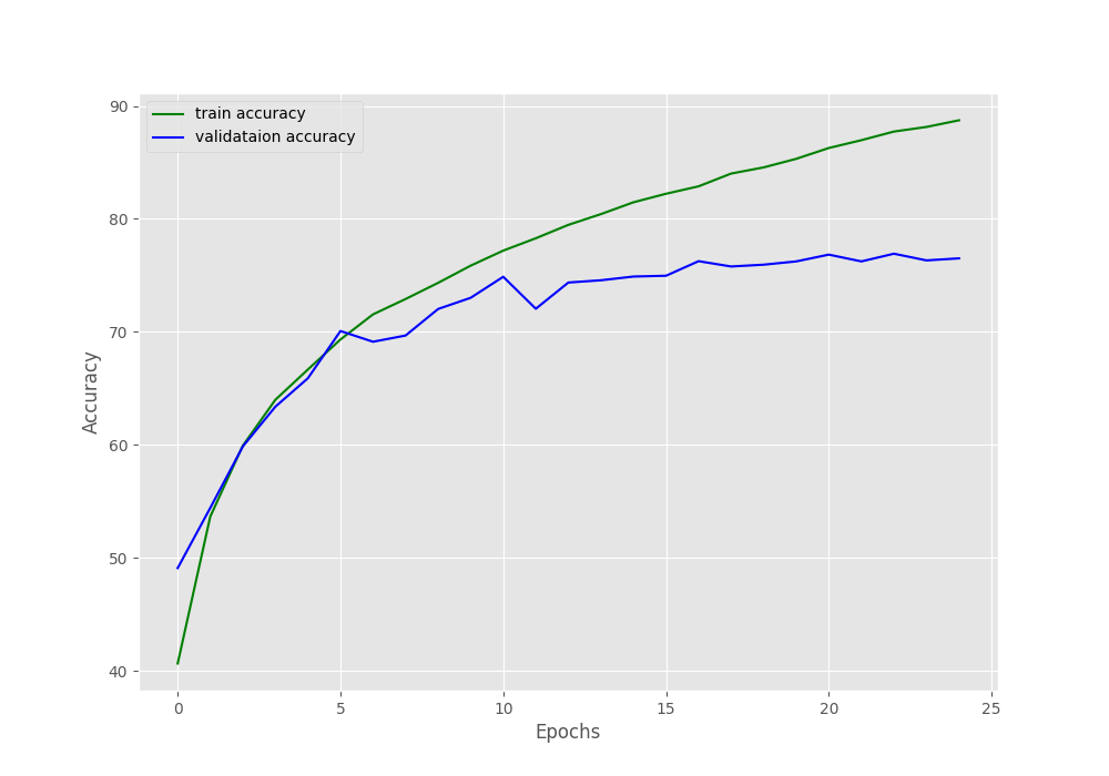
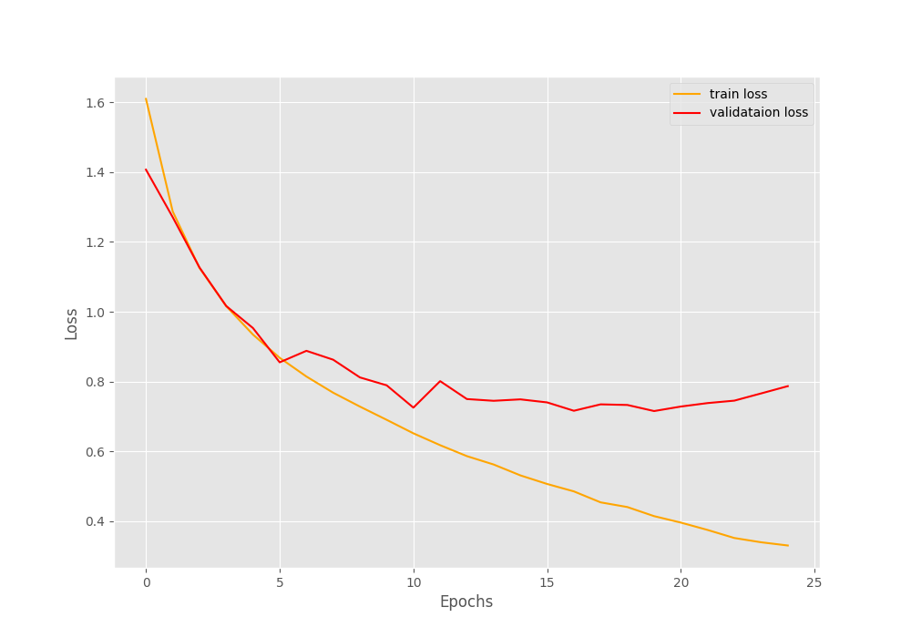
Although the validation and training accuracy is increasing till the end of the training, the validation loss is increasing after epoch 20. This indicates overfitting, and the last epoch’s model weights are not the best one for sure.

We can only confirm this if we test our best model weights and last epoch’s model weights on the test dataset. Let’s do that in the next section.

Testing the Best Weights and Last Epoch Saved Weights

In this section, we will write a test script to test our saved model weights. We will follow these steps:

• We will load both the available weights that we have saved to disk, the best ones, and from the last epoch as well.
• Then we will prepare the test data loader.
• In the next step, we will write a simple function that accepts a PyTorch model and a data loader as parameter. This will be the test function that will do only forward pass through the test data loader and give the final accuracy.
• We will pass both, the best saved model and last epoch saved model to the test function and compare the results.

Let’s start writing the code in the test.py script.

The first code block for the script sets all the import statements and the computation device.

import torch

from tqdm.auto import tqdm
from model import build_model
from datasets import create_datasets, create_data_loaders

# computation device
device = ('cuda' if torch.cuda.is_available() else 'cpu')
print(f"Computation device: {device}\n")

Build the Model and Load Both the Model Weights

Here, we will first build the ResNet18 model, and then load both sets of checkpoint files from the disk.

# build the model, no need to load the pre-trained weights or fine-tune layers
model = build_model(
    pretrained=False, fine_tune=False, num_classes=10
).to(device)
# load the best model checkpoint
best_model_cp = torch.load('outputs/best_model.pth')
best_model_epoch = best_model_cp['epoch']
print(f"Best model was saved at {best_model_epoch} epochs\n")

# load the last model checkpoint
last_model_cp = torch.load('outputs/final_model.pth')
last_model_epoch = last_model_cp['epoch']
print(f"Last model was saved at {last_model_epoch} epochs\n")

# get the test dataset and the test data loader
train_dataset, valid_dataset, test_dataset = create_datasets()
_, _, test_loader = create_data_loaders(
    train_dataset, valid_dataset, test_dataset
)

As we can see, after loading the checkpoints, we are extracting the epoch information from them and printing them. This is just to ensure that everything was loaded properly and we are in fact loading the correct checkpoints.

Starting from line 25, we prepare the test dataset and data loader.

The Test Function

The function to test the models by iterating over the test loader is very similar to the validation function that we used during the training.

def test(model, testloader):
    """
    Function to test the model
    """
    # set model to evaluation mode
    model.eval()
    print('Testing')
    valid_running_correct = 0
    counter = 0
    with torch.no_grad():
        for i, data in tqdm(enumerate(testloader), total=len(testloader)):
            counter += 1
            
            image, labels = data
            image = image.to(device)
            labels = labels.to(device)
            # forward pass
            outputs = model(image)
            # calculate the accuracy
            _, preds = torch.max(outputs.data, 1)
            valid_running_correct += (preds == labels).sum().item()
        
    # loss and accuracy for the complete epoch
    final_acc = 100. * (valid_running_correct / len(testloader.dataset))
    return final_acc

The only difference here from the validation function is that we are not calculating the loss. Just the accuracy which we are returning at the end as well.

There are two other functions. One to test the best model and the other to test the last epoch saved model. These two functions will actually load the weights into the ResNet18 architecture from the checkpoints and call the above test() function.

# test the last epoch saved model
def test_last_model(model, checkpoint, test_loader):
    print('Loading last epoch saved model weights...')
    model.load_state_dict(checkpoint['model_state_dict'])
    test_acc = test(model, test_loader)
    print(f"Last epoch saved model accuracy: {test_acc:.3f}")

# test the best epoch saved model
def test_best_model(model, checkpoint, test_loader):
    print('Loading best epoch saved model weights...')
    model.load_state_dict(checkpoint['model_state_dict'])
    test_acc = test(model, test_loader)
    print(f"Best epoch saved model accuracy: {test_acc:.3f}")

The above two functions look a bit redundant and can be reduced to just one function with a simple if block. But let’s stick to this approach, for now, to keep things simple.

Finally, we just need to call the test_last_model() and test_best_model() functions by passing the correct arguments.

if __name__ == '__main__':
    test_last_model(model, last_model_cp, test_loader)
    test_best_model(model, best_model_cp, test_loader)

The next step will be to execute the test.py script.

Execute test.py to Test the Models

From the same working directory, execute the following command in the terminal.

python test.py

The following is the output.

Computation device: cuda

[INFO]: Not loading pre-trained weights
[INFO]: Freezing hidden layers...
Best model was saved at 20 epochs

Last model was saved at 25 epochs

Files already downloaded and verified
Files already downloaded and verified
Files already downloaded and verified
Total training images: 40000
Total validation images: 10000
Total test images: 10000
Loading last epoch saved model weights...
Testing
100%|█████████████████████████████████████████████████████████████████████████████| 157/157 [00:03<00:00, 46.36it/s]
Last epoch saved model accuracy: 75.390
Loading best epoch saved model weights...
Testing
100%|█████████████████████████████████████████████████████████████████████████████| 157/157 [00:02<00:00, 78.30it/s]
Best epoch saved model accuracy: 76.060

The model weights from the last epoch gave us an accuracy of 75.390 and from the best epoch an accuracy of 76.60.

Although the difference is not huge, still, we can call it an improvement. Looks like using the best weights from the training actually helps. And please note that there is a chance that you may not get similar results as the training is not deterministic and we are not setting any seed here. But I hope that you get the idea and importance of saving the best model weights while training.

A Few Takeaways and Further Experiments

• There are a few loopholes to the above experiment in saving the best model in PyTorch. If you train for even longer with the current settings and parameters, then the model will overfit even more. And then if you run the test script again, there is a very high chance that the last epoch model will give more accuracy. The reason is that the test data is from the same distribution as the training data. So, in a way, the model would have memorized the dataset and therefore, give more accuracy. But that model will not be generalizable at all. If you find a few images from the internet, say, belonging to the horse class, then the model may not be able to predict those classes correctly. Therefore, if you want to train longer, then consider adding a whole lot of regularization. These can include, learning rate schedulers, more data augmentations, or even writing a custom model more suited towards the CIFAR10 dataset.
• Another experiment can be to try out ImageNet pre-trained weihgts and fine tuning the weights. It would be interesting to see how they perform.

If you carry out the above experiments, then let us know in the comment section.

Summary and Conclusion

In this tutorial, we saw how saving the best model in PyTorch while training can give better results during testing. We also discussed some of the possible loopholes around the current approach and how to overcome them. I hope that this tutorial was helpful to you.

If you have any doubts, thoughts, or suggestions, please leave them in the comment section. I will surely address them.

You can contact me using the Contact section. You can also find me on LinkedIn, and Twitter.