Stanford Cars Classification using EfficientNet PyTorch

A few days ago, I got a request from one of the readers about whether I can write a tutorial on Standford Cars classification using PyTorch and EfficientNet. There is already a post on using the pretrained PyTorch EfficientNet models for inference. So, I thought it will be a good idea to cover transfer learning on a larger dataset. Keep reading if you want to know how to carry out Stanford Cars classification using EfficientNet and the PyTorch framework.

The recent versions of PyTorch already provide EfficientNet models. So, it is going to be very easy for us to fine-tune the models on a new dataset. Torchvision provides all the seven models, starting from EfficientNet_B0 to EfficientNet_B7. And all of them have been pretrained on the ImageNet dataset. For that reason, the model should be able to perform very well which contains lots of images of cars.

We will cover the following topics in this tutorial.

• First, we discuss the dataset, that is, the Stanford Cars Dataset.
• Second, we will go through the EfficientNet model that we will train in this tutorial.
• Then we will move on to the coding section of Stanford cars classification using EfficietNet and PyTorch. There, we will discuss the important parts of the code. We will go through the major details while skipping the general aspects of deep learning image classification.
• After training and validating the model, we will visualize the Class Activation Maps (CAM) of the validation images.
• Finally, we will discuss some of the next steps to take to make this little project even better.

Let’s get into the technical details of the tutorial now.

The Stanford Cars Dataset

We will use the Stanford Cars dataset for fine-tuning the PyTorch EfficientNet model in this tutorial.

The dataset contains 16,185 images distributed over 196 classes. There are 8,144 images for training and 8,041 images for testing in this dataset. Each class roughly has a 50-50 split in the training and validation set.

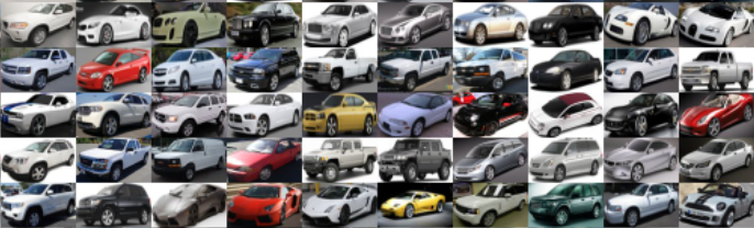
In the dataset, you will find the class names in the Make, Model, Year format. For example, an image may have Acura Integra Type R 2001 as the class name.

Although the dataset is available on its official website, we will not download it from there. Rather, we will download the dataset from Kaggle. This version of the dataset already has all the images in the proper training and validation folders. For that reason, we will not have to focus much on the data preparation part.

For now, you can download the dataset and extract it. After extracting it, you should get the following directory structure.

├── car_data
│   └── car_data
│       ├── test
│       │   ├── Acura Integra Type R 2001
│       │   ├── Acura RL Sedan 2012
│       │   ├── Acura TL Sedan 2012
│       │   ├── Acura TL Type-S 2008
│       │   ├── Acura TSX Sedan 2012
│       │   ├── Acura ZDX Hatchback 2012
│       │   ├── AM General Hummer SUV 2000
│       │   ├── Aston Martin V8 Vantage Convertible 2012
│       │   ├── Aston Martin V8 Vantage Coupe 2012
│       │   ├── Aston Martin Virage Convertible 2012
│       │   ...
│       └── train
│           ├── Acura Integra Type R 2001
│           ├── Acura RL Sedan 2012
│           ├── Acura TL Sedan 2012
│           ├── Acura TL Type-S 2008
│           ...
│           ├── Volvo C30 Hatchback 2012
│           └── Volvo XC90 SUV 2007
├── anno_test.csv
├── anno_train.csv
└── names.csv

The images are present in the respective class folders in the train and test directories. The dataset also contains a few CSV files but we will not be needing those. In one of the following sections, we will check out how to structure the directory for the entire tutorial.

The PyTorch EfficientNet B1 Model

We will use the EfficientNet B1 model for the Stanford Cars classification in this tutorial. The pretrained EfficientNet B1 model is available with the torchvision library along with the other models of the family. As it has been pretrained on the ImageNet dataset, by default it has 1000 units in the final linear layer. We will change that. Also, currently, it has 7,794,184 parameters. As our dataset contains 196 classes, the final model that we will use will have fewer parameters. Somewhere around 6 million parameters.

Directory Structure for The Project

The following block shows the directory structure for the entire project.

├── input
│   ├── car_data
│   │   └── car_data
│   │       ├── test
│   │       └── train
│   ├── anno_test.csv
│   ├── anno_train.csv
│   └── names.csv
├── outputs
│   ├── cam_results [8041 entries exceeds filelimit, not opening dir]
│   ├── accuracy.png
│   ├── loss.png
│   └── model.pth
├── src
    ├── cam.py
    ├── class_names.py
    ├── datasets.py
    ├── model.py
    ├── train.py
    └── utils.py

We have already seen the structure of the input directory. Going over the other directories and files:

• The outputs directory holds all the results that we will get from training and testing the model. This includes the loss & accuracy graphs, and the trained model as well. It has a cam_results subdirectory also which holds the Class Activation Map results along with the ground truth and predicted labels for all the images in the test directory. Note that we will use the images from the test directory as validation images.
• The src directory contains the Python files that we need in this tutorial. We will get to know their details in the coding section.

You can download the zip file for this tutorial which provides all the training scripts and the trained model as well.

Stanford Cars Classification Using EfficientNet B1 and PyTorch

Let’s go through the important coding section of this tutorial. We will cover all the code here so that anyone reading through can go through the code, but we will get into the explanation of the important parts only. This is because a lot of it is simple code for image classification.

We will carry out the training of the model first and then the inference with visualization of the Class Activation Maps. So, first, we will go through all the code that we need for training the model.

With that in mind, let’s start.

Note that all the Python files are present in the src directory.

The Utilities and Helper Functions

We have two helper functions. One is for saving the model to disk, and the other one is for saving the loss & accuracy graphs.

The helper functions are part of the utils.py file.

The following code block contains both of the functions.

import torch
import matplotlib
import matplotlib.pyplot as plt

matplotlib.style.use('ggplot')

def save_model(epochs, model, optimizer, criterion):
    """
    Function to save the trained model to disk.
    """
    torch.save({
                'epoch': epochs,
                'model_state_dict': model.state_dict(),
                'optimizer_state_dict': optimizer.state_dict(),
                'loss': criterion,
                }, f"../outputs/model.pth")

def save_plots(train_acc, valid_acc, train_loss, valid_loss):
    """
    Function to save the loss and accuracy plots to disk.
    """
    # Accuracy plots.
    plt.figure(figsize=(10, 7))
    plt.plot(
        train_acc, color='green', linestyle='-', 
        label='train accuracy'
    )
    plt.plot(
        valid_acc, color='blue', linestyle='-', 
        label='validataion accuracy'
    )
    plt.xlabel('Epochs')
    plt.ylabel('Accuracy')
    plt.legend()
    plt.savefig(f"../outputs/accuracy.png")
    
    # Loss plots.
    plt.figure(figsize=(10, 7))
    plt.plot(
        train_loss, color='orange', linestyle='-', 
        label='train loss'
    )
    plt.plot(
        valid_loss, color='red', linestyle='-', 
        label='validataion loss'
    )
    plt.xlabel('Epochs')
    plt.ylabel('Loss')
    plt.legend()
    plt.savefig(f"../outputs/loss.png")

Both of the above functions are very general ones. One thing to note here is that we are saving the epoch, optimizer, and loss function information as well while saving the model weights. This can potentially be helpful when trying to resume training later on.

Preparing the Datasets

Next is preparing the dataset and data loaders. This section should be pretty much straightforward as we already have the training and validation images in separate folders.

The dataset preparation code will go into the datasets.py file.

Let’s start with the imports and define a few constants that we need for the dataset preparation.

from torchvision import datasets, transforms
from torch.utils.data import DataLoader

# Required constants.
TRAIN_DIR = '../input/car_data/car_data/train/'
VALID_DIR = '../input/car_data/car_data/test/'
IMAGE_SIZE = 224 # Image size of resize when applying transforms.
BATCH_SIZE = 32
NUM_WORKERS = 4 # Number of parallel processes for data preparation.

For the constants, we have, TRAIN_DIR and VALID_DIR defining the training and validation image paths. We also define the IMAGE_SIZE for resizing the image while applying the transforms. And then the batch size and number of workers for the data loaders.

Now, let’s define the training and validation transforms.

# Training transforms
def get_train_transform(IMAGE_SIZE):
    train_transform = transforms.Compose([
        transforms.Resize((IMAGE_SIZE, IMAGE_SIZE)),
        transforms.RandomHorizontalFlip(p=0.5),
        transforms.RandomRotation(35),
        transforms.RandomAdjustSharpness(sharpness_factor=2, p=0.5),
        transforms.RandomGrayscale(p=0.5),
        transforms.RandomPerspective(distortion_scale=0.5, p=0.5),
        transforms.RandomPosterize(bits=2, p=0.5),
        transforms.ToTensor(),
        transforms.Normalize(
            mean=[0.485, 0.456, 0.406],
            std=[0.229, 0.224, 0.225]
            )
    ])
    return train_transform

# Validation transforms
def get_valid_transform(IMAGE_SIZE):
    valid_transform = transforms.Compose([
        transforms.Resize((IMAGE_SIZE, IMAGE_SIZE)),
        transforms.ToTensor(),
        transforms.Normalize(
            mean=[0.485, 0.456, 0.406],
            std=[0.229, 0.224, 0.225]
            )
    ])
    return valid_transform

We can see that the get_train_transform function contains a lot of augmentations. These include pixel color as well as spatial transforms. It is mainly to avoid overfitting while training. While training, the model was overfitting pretty quickly without any augmentations. The above augmentations help to prevent overfitting too soon and give the validation accuracy a chance to increase for a larger number of epochs. We don’t need any augmentations for the validation data.

For the normalization, we are using the ImageNet stats as we will be fine-tuning an ImageNet pretrained EfficientNet B1 model.

Finally, we write the functions to prepare the dataset and data loaders for training as well as validation.

def get_datasets():
    """
    Function to prepare the Datasets.
    Returns the training and validation datasets along 
    with the class names.
    """
    dataset_train = datasets.ImageFolder(
        TRAIN_DIR, 
        transform=(get_train_transform(IMAGE_SIZE))
    )
    dataset_valid = datasets.ImageFolder(
        VALID_DIR, 
        transform=(get_valid_transform(IMAGE_SIZE))
    )
    return dataset_train, dataset_valid, dataset_train.classes

def get_data_loaders(dataset_train, dataset_valid):
    """
    Prepares the training and validation data loaders.
    :param dataset_train: The training dataset.
    :param dataset_valid: The validation dataset.
    Returns the training and validation data loaders.
    """
    train_loader = DataLoader(
        dataset_train, batch_size=BATCH_SIZE, 
        shuffle=True, num_workers=NUM_WORKERS
    )
    valid_loader = DataLoader(
        dataset_valid, batch_size=BATCH_SIZE, 
        shuffle=False, num_workers=NUM_WORKERS
    )
    return train_loader, valid_loader 

The get_datasets function prepares and returns the training and validation datasets. Similarly, the get_data_loaders function returns the respective data loaders.

The EfficientNet B1 Model

The model preparation is going to be easy. As Torchvision already provides the pretrained model, we just need to change the final classification head according to our dataset.

The following code will go into the model.py file.

import torch.nn as nn

from torchvision import models

def build_model(pretrained=True, fine_tune=True, num_classes=10):
    if pretrained:
        print('[INFO]: Loading pre-trained weights')
    else:
        print('[INFO]: Not loading pre-trained weights')
    model = models.efficientnet_b1(pretrained=pretrained)

    if fine_tune:
        print('[INFO]: Fine-tuning all layers...')
        for params in model.parameters():
            params.requires_grad = True
    elif not fine_tune:
        print('[INFO]: Freezing hidden layers...')
        for params in model.parameters():
            params.requires_grad = False

    # Change the final classification head.
    model.classifier[1] = nn.Linear(in_features=1280, out_features=num_classes)
    return model

We load the efficientnet_b1 model with the pretrained weights on line 10. Lines 12 to 19 set the weights as either trainable or non-trainable as per the fine_tune parameter. Then we change the number of input features in the final Linear layer on line 22. And that’s all we need to do to prepare the model.

The Training Script

Before we can start the training, we need to write the code for the executable training script.

This code is part of the train.py script. It combines together all that we have been doing till now.

First, we will import all the required modules, set the seed for reproducibility, and construct the argument parser.

import torch
import argparse
import torch.nn as nn
import torch.optim as optim
import time

from tqdm.auto import tqdm

from model import build_model
from datasets import get_datasets, get_data_loaders
from utils import save_model, save_plots

seed = 42
torch.manual_seed(seed)
torch.cuda.manual_seed(seed)
torch.backends.cudnn.deterministic = True
torch.backends.cudnn.benchmark = True

# Construct the argument parser.
parser = argparse.ArgumentParser()
parser.add_argument(
    '-e', '--epochs', type=int, default=10,
    help='Number of epochs to train our network for'
)
parser.add_argument(
    '-lr', '--learning-rate', type=float,
    dest='learning_rate', default=0.001,
    help='Learning rate for training the model'
)
args = vars(parser.parse_args())

For the argument parser, we have the following flags:

• --epochs: To set the number of epochs to train for.
• --learning-rate: Different models may require different learning rates depending upon the size and whether we use pretrained weights or not. This flag will be helpful to set the learning rate dynamically.

The Training and Validation Functions

Now, we define the function for completing one epoch of training.

# Training function.
def train(model, trainloader, optimizer, criterion):
    model.train()
    print('Training')
    train_running_loss = 0.0
    train_running_correct = 0
    counter = 0
    for i, data in tqdm(enumerate(trainloader), total=len(trainloader)):
        counter += 1
        image, labels = data
        image = image.to(device)
        labels = labels.to(device)
        optimizer.zero_grad()
        # Forward pass.
        outputs = model(image)
        # Calculate the loss.
        loss = criterion(outputs, labels)
        train_running_loss += loss.item()
        # Calculate the accuracy.
        _, preds = torch.max(outputs.data, 1)
        train_running_correct += (preds == labels).sum().item()
        # Backpropagation.
        loss.backward()
        # Update the weights.
        optimizer.step()
    
    # Loss and accuracy for the complete epoch.
    epoch_loss = train_running_loss / counter
    epoch_acc = 100. * (train_running_correct / len(trainloader.dataset))
    return epoch_loss, epoch_acc 

It is a simple function that accepts the model, the training data loader, the optimizer, and the loss function. It returns the loss value and accuracy after training on the entire dataset on each epoch.

Similarly, we have the validation function.

# Validation function.
def validate(model, testloader, criterion, class_names):
    model.eval()
    print('Validation')
    valid_running_loss = 0.0
    valid_running_correct = 0
    counter = 0

    with torch.no_grad():
        for i, data in tqdm(enumerate(testloader), total=len(testloader)):
            counter += 1
            
            image, labels = data
            image = image.to(device)
            labels = labels.to(device)
            # Forward pass.
            outputs = model(image)
            # Calculate the loss.
            loss = criterion(outputs, labels)
            valid_running_loss += loss.item()
            # Calculate the accuracy.
            _, preds = torch.max(outputs.data, 1)
            valid_running_correct += (preds == labels).sum().item()
        
    # Loss and accuracy for the complete epoch.
    epoch_loss = valid_running_loss / counter
    epoch_acc = 100. * (valid_running_correct / len(testloader.dataset))
    return epoch_loss, epoch_acc

For the validation, we don’t need any backpropagation or updating of the model parameters.

The Main Training Block

Finally, we need the main training block. Let’s write the entire code first and then get into the important parts.

if __name__ == '__main__':
    # Load the training and validation datasets.
    dataset_train, dataset_valid, dataset_classes = get_datasets()
    print(f"[INFO]: Number of training images: {len(dataset_train)}")
    print(f"[INFO]: Number of validation images: {len(dataset_valid)}")
    # Load the training and validation data loaders.
    train_loader, valid_loader = get_data_loaders(dataset_train, dataset_valid)

    # Learning_parameters. 
    lr = args['learning_rate']
    epochs = args['epochs']
    device = ('cuda' if torch.cuda.is_available() else 'cpu')
    print(f"Computation device: {device}")
    print(f"Learning rate: {lr}")
    print(f"Epochs to train for: {epochs}\n")

    # Load the model.
    model = build_model(
        pretrained=True,
        fine_tune=True, 
        num_classes=len(dataset_classes)
    ).to(device)
    
    # Total parameters and trainable parameters.
    total_params = sum(p.numel() for p in model.parameters())
    print(f"{total_params:,} total parameters.")
    total_trainable_params = sum(
        p.numel() for p in model.parameters() if p.requires_grad)
    print(f"{total_trainable_params:,} training parameters.")

    # Optimizer.
    optimizer = optim.Adam(model.parameters(), lr=lr)
    # Loss function.
    criterion = nn.CrossEntropyLoss()

    # Lists to keep track of losses and accuracies.
    train_loss, valid_loss = [], []
    train_acc, valid_acc = [], []
    # Start the training.
    for epoch in range(epochs):
        print(f"[INFO]: Epoch {epoch+1} of {epochs}")
        train_epoch_loss, train_epoch_acc = train(model, train_loader, 
                                                optimizer, criterion)
        valid_epoch_loss, valid_epoch_acc = validate(model, valid_loader,  
                                                    criterion, dataset_classes)
        train_loss.append(train_epoch_loss)
        valid_loss.append(valid_epoch_loss)
        train_acc.append(train_epoch_acc)
        valid_acc.append(valid_epoch_acc)
        print(f"Training loss: {train_epoch_loss:.3f}, training acc: {train_epoch_acc:.3f}")
        print(f"Validation loss: {valid_epoch_loss:.3f}, validation acc: {valid_epoch_acc:.3f}")
        print('-'*50)
        time.sleep(2)

    # Save the trained model weights.
    save_model(epochs, model, optimizer, criterion)
    # Save the loss and accuracy plots.
    save_plots(train_acc, valid_acc, train_loss, valid_loss)
    print('TRAINING COMPLETE')

Going over the above code block:

• First, we prepare the datasets and data loaders.
• Second, we set all the learning parameters like the learning rate, number of epochs, and also the computation device.
• Then we initialize the model. Note that we are providing fine_tune=True indicating that we will be retraining all the model weights.
• Then we set the optimizer and the loss function.
• Finally, we have the training loop where we print the loss and accuracy values after each epoch. After the training ends, we save the model and the loss & accuracy graphs to disk.

We have completed all the code that we need for training and are all set to train the model.

Training the PyTorch EfficientNet B1 Model on the Stanford Cars Dataset

All training and inference experiments are done on a system with 32 GB RAM, an i7 10th Generation CPU, and an RTX 3080 GPU with 10 GB of VRAM.

For training the model, we need to execute the following command from the terminal within the src directory.

python train.py --epochs 50 --learning-rate 0.0001

We are training the model for 50 epochs with a learning rate of 0.0001.

The following block shows the truncated results.

[INFO]: Number of training images: 8144
[INFO]: Number of validation images: 8041
Computation device: cuda
Learning rate: 0.0001
Epochs to train for: 50

[INFO]: Loading pre-trained weights
[INFO]: Fine-tuning all layers...
6,764,260 total parameters.
6,764,260 training parameters.
[INFO]: Epoch 1 of 50
Training
100%|██████████████████████████████████████████████████████████████████| 255/255 [00:25<00:00,  9.92it/s]
Validation
100%|██████████████████████████████████████████████████████████████████| 252/252 [00:11<00:00, 22.72it/s]
Training loss: 5.274, training acc: 0.921
Validation loss: 5.178, validation acc: 2.624
--------------------------------------------------
.
.
.
[INFO]: Epoch 50 of 50
Training
100%|██████████████████████████████████████████████████████████████████| 255/255 [00:24<00:00, 10.54it/s]
Validation
100%|██████████████████████████████████████████████████████████████████| 252/252 [00:10<00:00, 23.77it/s]
Training loss: 0.143, training acc: 96.022
Validation loss: 0.576, validation acc: 84.679
--------------------------------------------------
TRAINING COMPLETE

By the end of 50 epochs, the validation accuracy hovers somewhere around 84.2% to 84.7%. And the validation loss is somewhere around 0.57. The training accuracy is much higher and loss is also lower.

Perhaps, taking a look at the graphs will give us more insights.

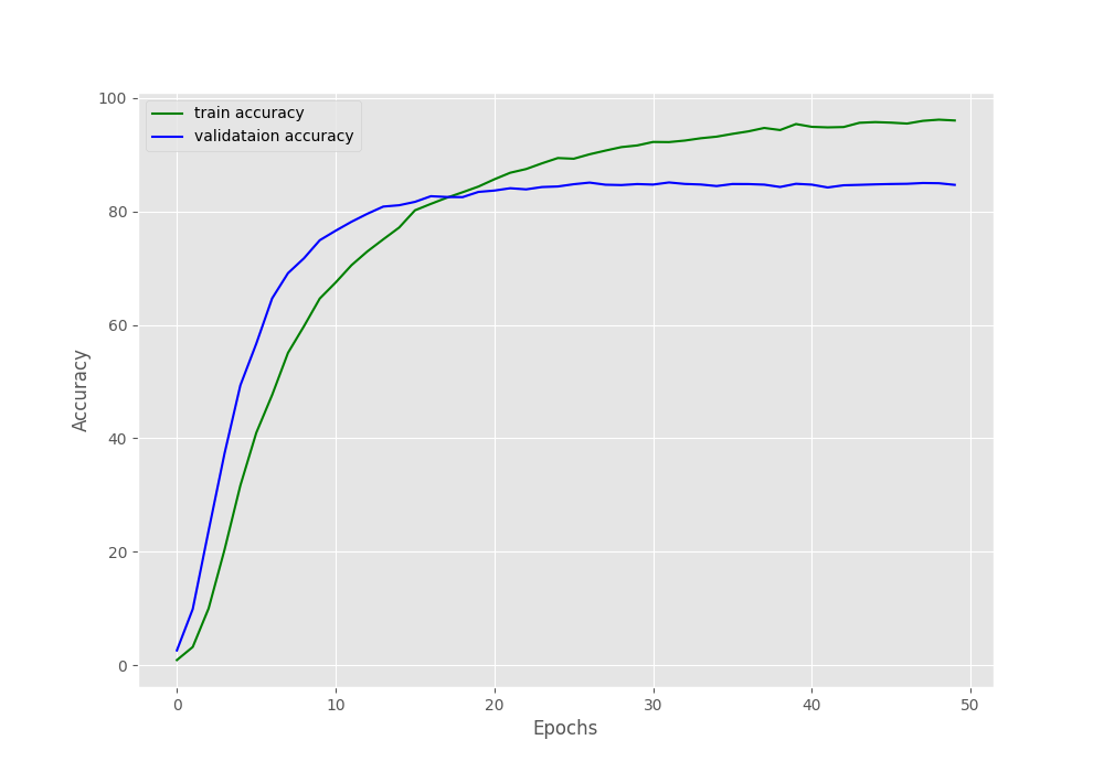
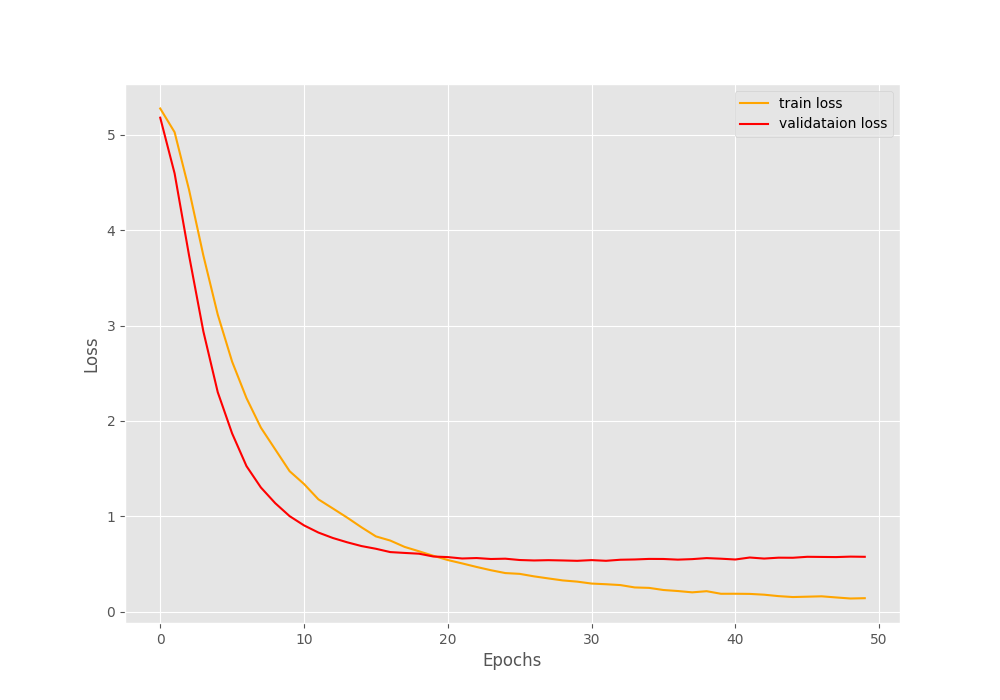
If we observe the validation loss line properly, we can see some slight overfitting at the end of the training. Training any more would surely lead to even more overfitting and the model may lose its ability to generalize. We will discuss some of the potential steps that we can take to prevent such a scenario.

Carrying Out Inference and Visualizing Class Activation Maps

For the final coding part of this post, we will carry out inference on all the validation images again. Along with that, we will cover the following things:

• Visualize the Class Activation Maps (CAM) of all the predictions.
• Observe the total number of correct predictions out of the 8041 validation images.
• Calculate the average FPS of the EfficientNet B1 model for going through all the images.

All the above mentioned points are carried out by the code available in cam.py script.

We will not go through the code here. You can find all the Class Activation Map related posts (theory and coding) in the following tutorials:

• Basic Introduction to Class Activation Maps in Deep Learning using PyTorch
• Saliency Maps in Convolutional Neural Networks
• PyTorch Class Activation Map using Custom Trained Model

The code in this post is slightly modified compared to the ones in the above list. Going through the code will clarify those parts for sure.

Let’s execute the cam.py script and check out the results.

python cam.py 

The outputs should be similar to the following.

[INFO]: Not loading pre-trained weights
[INFO]: Freezing hidden layers...
EfficientNet(
  (features): Sequential(
.
.
.
Image: 8041
Total number of test images: 8041
Total correct predictions: 6809
Accuracy: 84.679
Average FPS: 54.161

The above results will be very similar to the ones that we got in the validation loops while training as we are using the same validation data here. The trained model predicts the classes of 6809 images correctly which accounts for 84.67% accuracy. And the average FPS on the RTX 3080 GPU is around 54.

The Class Activation Map Results

Now, let’s take a look at some of the results that are saved to the outputs/cam_results. This will give us a good idea of the mistakes that the model is making and what part of a car it is focusing on during the predictions.

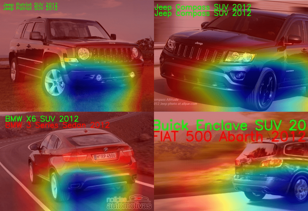
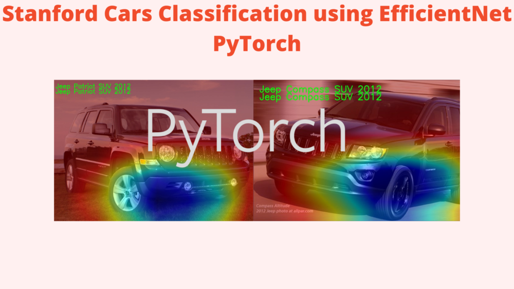
In the above figure, the text on top of each image is the ground truth label and the text below that is the predicted label. If the model is predicting the label correctly, we are showing that in green color, else we are showing that in red color.

The model is predicting the two SUVs correctly. In this case, the model is focusing on the headlights, the area around the front grille, and the side of the car. If we observe closely, the red activation map is also encompassing the model text on both the SUVs. So, the model may be getting some hints from those.

In one of the incorrect predictions, the model is making the wrong prediction for the model of the car. However, it is correctly predicting the make (BMW) of the car and obviously, we can see that the heat map is being concentrated around the logo in this case.

The other wrong prediction is wrong for both, the make and the model as well. Although the model is looking entirely at one side of the car, perhaps, the prediction is wrong because the logo is unclear. Clearly, this is a limitation, as a properly trained model will be able to predict it correctly from other parts of the car as well.

Improving the Model Further

Here are a few options that one may consider for improving the results of Stanford Cars classification using EfficientNet B1 even further.

• Adding more geometric augmentation: This may help to prevent the overfitting around the final few epochs that we faced.
• Adding learning rate scheduler: Using a learning rate scheduler will surely help to prevent overfitting and help train even longer.
• Saving the best model only: We can also save the best model weights instead of the last ones (which may be the overfit weights). You may refer to this tutorial to learn how to do that with PyTorch.

Summary and Conclusion

In this tutorial, we went through a small project of Stanford Cars classification using the EfficientNet B1 model with the PyTorch deep learning framework. We also checked out the inference results along with the Class Activation Maps. Finally, we discussed some of the potential improvements that we can add to the training process. I hope that this tutorial was helpful to you.

If you have any doubts, thoughts, or suggestions, please leave them in the comment section. I will surely address them.

You can contact me using the Contact section. You can also find me on LinkedIn, and Twitter.