PyTorch Class Activation Map using Custom Trained Model

In this tutorial, you will learn how to visualize class activation map in PyTorch using a custom trained model.

We often describe neural networks as black boxes as it is hard to interpret their decisions. But that is slowly changing over the years with the introduction of neural network interpretation techniques. Saliency maps, class activation maps (CAM), and Grad-CAM are some of them.

In one of the previous tutorials, we used a pre-trained PyTorch model to visualize the class activation map (CAM) on a set of images. The model was trained on the ImageNet dataset and therefore was able to predict the classes of thousands of images correctly. In another post, we went over a few network interpretation techniques in brief. We discussed a few papers and the techniques introduced by them.

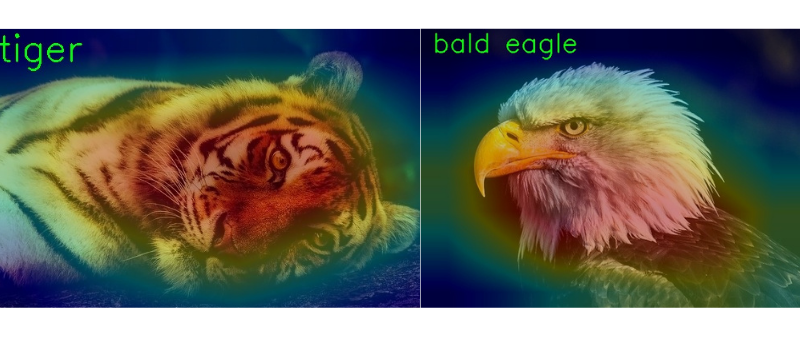
Figure 1 shows some of the outputs from one of the previous posts for class activation map.

For this tutorial, we will visualize the class activation map in PyTorch using a custom trained model.

• We will train a small convolutional neural network on the Digit MNIST dataset.
• The model will be small and simple. Also, the training and validation pipeline will be pretty basic.
• Our main focus will be to load the trained model, feed it with a new set of unseen images, and see what it classifies those images as and why it classifies them so.

Overall, this should be a good exercise to start exploring neural network model interpretability for custom trained models. Then we can apply this process to many larger projects further on.

Directory Structure

Let’s take a look at the directory structure that we will use for this project.

├── data
│   └── MNIST
├── input
│   ├── eight.png
│   ├── five.png
│   ...
├── outputs
│   ├── CAM_eight.jpg
│   ├── CAM_five.jpg
│   ...
├── cam.py
├── model.py
└── train_mnist.py

• The data folder contains the MNIST dataset. This will get automatically downloaded when we will prepare the dataset while writing the PyTorch code.
• The input folder contains the test images. These are a few digit images that I have created manually. You will find these when you download the project zip file. We will use these images to test the trained model. This will give us a good idea why the trained model predicted a certain label for a digit and also at what part of the digit it was looking at.
• All the prediction results from the test phase will go into the outputs folder.
• The model.py Python file contains the neural network architecure. It is a simple convolutional neural network.
• The train_mnist.py is the executable script that we will use to train and validate the neural network model on the MNIST dataset.
• Finally, the cam.py is the test script. We will use this to predict the class labels for the test images and visualize the class activation maps as well.

If you want to explore the scripts a bit after downloading the project file, feel free to do so. It will make the understanding of the code easier later on. From the next section onward, we will start with the coding part of this tutorial.

Visualizing Class Activation Map in PyTorch using Custom Trained Model

Let’s get into the coding part without any further delay. Essentially, we have three parts here:

• First, we will define the neural network model.
• Second, we will write the training script to train the neural network model on the MNIST dataset.
• Third, we will use the trained model to classify and visualize the class activation map using PyTorch on new and unseen images.

The Neural Network Model

The neural network architecture code will go into the model.py Python file.

The following code block contains the entire neural network model architecture code.

import torch
import torch.nn as nn

class Net(nn.Module):
    def __init__(self):
        super(Net, self).__init__()
        self.conv = nn.Sequential(
            nn.Conv2d(1, 16, 5),
            nn.ReLU(),
            nn.MaxPool2d(kernel_size=2),
            nn.Conv2d(16, 32, 4),
            nn.ReLU(),
            nn.MaxPool2d(kernel_size=2)
        )
        self.linear = nn.Sequential(
            nn.Linear(32 * 4 * 4, 32),
            nn.ReLU(),
            nn.Linear(32, 10)
        )

    def forward(self, x):
        x = self.conv(x)
        x = torch.flatten(x, 1)
        x = self.linear(x)
        return x

As you can see, it is a very simple architecture.

• The self.conv variable holds the first Sequential block. This consists of two convolutional layers each followed by the ReLU activation and MaxPool2D.
• Then the self.linear variable holds all the linear layers of the model. As usual, the last linear layer has 10 output features corresponding to the 10 classes in the MNIST dataset.

Dividing the entire model into separate modules like the above actually helps a lot. The self.conv block will act as the feature extractor as it has only the convolutional layers. While writing the code for class activation map, we will need these features and it will be very easy for us to do that when we build the architecture as above. We can easily access the convolutional features using PyTorch hooks. This will become even more clear when we reach that part and write the code.

For now, let’s start with the training code.

The Training Script for PyTorch Class Activation Map

The code that we will write here will go into the train_mnist.py script.

Let’s start with the import statements.

import torch
import torchvision
import torchvision.transforms as transforms
import torch.nn as nn
import torch.optim as optim
import matplotlib.pyplot as plt
import matplotlib

from tqdm.auto import tqdm
from model import Net

matplotlib.style.use('ggplot')

We are importing everything we need like:

• torch to access the core functionalitues.
• torchvision to access and download the MNIST dataset, also transforms to apply the image transforms.
• We are importing the Net class from model module to initialize the model.

The next code block defines the computation device and the image transforms.

# define the computation device
device = ('cuda' if torch.cuda.is_available() else 'cpu')

# image augmentations and transforms...
# ... we are coverting to tensor and normalizing the pixels
transform = transforms.Compose(
    [transforms.ToTensor(),
     transforms.Normalize((0.5), (0.5))])

For the training, either GPU or CPU will work fine. MNIST is not a computation heavy dataset and neither is our model. You can very easily train on a CPU as well.

For the image transforms, we are just converting the images to tensors and normalizing the pixels. We will use the same transform for both training and validation data loaders. Let’s keep things simple and focus on class activation map visualization.

Training and Validation Dataloaders

Next, let’s prepare the training and validation data loaders.

# define the batch size for data loaders
batch_size = 256
# training dataset and data loader
train_dataset = torchvision.datasets.MNIST(root='./data', train=True,
                                        download=True, transform=transform)
trainloader = torch.utils.data.DataLoader(train_dataset, batch_size=batch_size,
                                          shuffle=True, num_workers=2)
# validation dataset and data loader
valid_dataset = torchvision.datasets.MNIST(root='./data', train=False,
                                       download=True, transform=transform)
validloader = torch.utils.data.DataLoader(valid_dataset, batch_size=batch_size,
                                         shuffle=False, num_workers=2)

We are using a batch size of 256. From experimentations, I found that without augmentations, a batch size of 256 results in more stable training than smaller batches. For MNIST data, this should work perfectly fine without any memory errors as the images are just 28×28 in dimensions.

We are loading the MNIST data directly from the torchvision.datasets module and applying the transform.

For both, trainloader and validloader, we are using num_workers as 2. If you face BrokenPipeError, then consider making the value as 0 and everything should work well. This most likely happens when running on Windows, but as it seems this problem has been solved with the latest PyTorch version.

Initialize the Model, Loss Function, and Optimizer

Now, we will initialize the mode and load it onto the computation device. For the loss function, we will use CrossEntropyLoss, and SGD (Stochastic Gradient Descent) as the optimizer.

# initialize model
model = Net()
# load on to computation device
model = model.to(device)
criterion = nn.CrossEntropyLoss()
optimizer = optim.SGD(model.parameters(), lr=0.01, momentum=0.9)

For the optimizer, the learning rate is 0.01 and the momentum is 0.9.

The Training Function

The training function, that is, train(), will accept the model, trainloader, optimizer, and criterion as the parameters.

The following code block contains the training function.

# training function
def train(model, trainloader, optimizer, criterion):
    model.train()
    print('Training')
    train_running_loss = 0.0
    train_running_correct = 0
    counter = 0
    for i, data in tqdm(enumerate(trainloader), total=len(trainloader)):
        counter += 1
        image, labels = data
        image = image.to(device)
        labels = labels.to(device)
        optimizer.zero_grad()
        # forward pass
        outputs = model(image)
        # calculate the loss
        loss = criterion(outputs, labels)
        train_running_loss += loss.item()
        # calculate the accuracy
        _, preds = torch.max(outputs.data, 1)
        train_running_correct += (preds == labels).sum().item()
        # backpropagation
        loss.backward()
        # update the optimizer parameters
        optimizer.step()
    
    # loss and accuracy for the complete epoch
    epoch_loss = train_running_loss / counter
    epoch_acc = 100. * (train_running_correct / len(trainloader.dataset))
    return epoch_loss, epoch_acc

It is a very standard training function for PyTorch image classification. After every epoch, the function returns the loss and accuracy values. We will not go into the details of the training function here.

The Validation Function

It will be very similar to the training function. But we will not backpropagate the gradients or update the optimizer parameters.

# validation function
def validate(model, testloader, criterion):
    model.eval()
    print('Validation')
    valid_running_loss = 0.0
    valid_running_correct = 0
    counter = 0
    with torch.no_grad():
        for i, data in tqdm(enumerate(testloader), total=len(testloader)):
            counter += 1
            image, labels = data
            image = image.to(device)
            labels = labels.to(device)
            # forward pass
            outputs = model(image)
            # calculate the loss
            loss = criterion(outputs, labels)
            valid_running_loss += loss.item()
            # calculate the accuracy
            _, preds = torch.max(outputs.data, 1)
            valid_running_correct += (preds == labels).sum().item()
        
    # loss and accuracy for the complete epoch
    epoch_loss = valid_running_loss / counter
    epoch_acc = 100. * (valid_running_correct / len(testloader.dataset))
    return epoch_loss, epoch_acc

Here too, we are returning the loss and accuracy values after every epoch.

The Training Loop

The training and validation functions are returning the respective loss and accuracy values after each epoch. We will create four lists and keep on appending the values after each epoch.

# lists to keep track of losses and accuracies
train_loss, valid_loss = [], []
train_acc, valid_acc = [], []
epochs = 30
# start the training
for epoch in range(epochs):
    print(f"[INFO]: Epoch {epoch+1} of {epochs}")
    train_epoch_loss, train_epoch_acc = train(model, trainloader, 
                                              optimizer, criterion)
    valid_epoch_loss, valid_epoch_acc = validate(model, validloader,  
                                                 criterion)
    train_loss.append(train_epoch_loss)
    valid_loss.append(valid_epoch_loss)
    train_acc.append(train_epoch_acc)
    valid_acc.append(valid_epoch_acc)
    print(f"Training loss: {train_epoch_loss:.3f}, training acc: {train_epoch_acc:.3f}")
    print(f"Validation loss: {valid_epoch_loss:.3f}, validation acc: {valid_epoch_acc:.3f}")
    print('-'*50)

print('TRAINING COMPLETE')

We are training for 30 epochs. This should be enough to give an accuracy of more than 99% on the MNIST dataset.

Finally, let’s write the code to plot the accuracy and loss line graph and save them in the outputs folder.

# accuracy plots
plt.figure(figsize=(10, 7))
plt.plot(
    train_acc, color='green', linestyle='-', 
    label='train accuracy'
)
plt.plot(
    valid_acc, color='blue', linestyle='-', 
    label='validataion accuracy'
)
plt.xlabel('Epochs')
plt.ylabel('Accuracy')
plt.legend()
plt.savefig('outputs/accuracy.png')
plt.show()
# loss plots
plt.figure(figsize=(10, 7))
plt.plot(
    train_loss, color='orange', linestyle='-', 
    label='train loss'
)
plt.plot(
    valid_loss, color='red', linestyle='-', 
    label='validataion loss'
)
plt.xlabel('Epochs')
plt.ylabel('Loss')
plt.legend()
plt.savefig('outputs/loss.png')
plt.show()

# save the final model
save_path = 'model.pth'
torch.save(model.state_dict(), save_path)
print('MODEL SAVED...')

In the end, we are also saving the trained model to disk with model.pth file name.

This ends all the code we need for training our simple neural network model on the MNIST dataset.

Execute train_mnist.py for Training

We are all set to execute the train_mnist.py script. Open up your terminal/command line in the current working directory. And type the following command.

python train_mnist.py

You should see output similar to the following.

[INFO]: Epoch 1 of 10
100%|███████████████████████████████████████████████████████████████| 235/235 [00:03<00:00, 66.57it/s]
Validation
100%|█████████████████████████████████████████████████████████████████| 40/40 [00:00<00:00, 68.99it/s]
Training loss: 0.719, training acc: 77.375
Validation loss: 0.142, validation acc: 95.570
--------------------------------------------------
[INFO]: Epoch 2 of 30
Training
100%|███████████████████████████████████████████████████████████████| 235/235 [00:03<00:00, 69.69it/s]
Validation
100%|█████████████████████████████████████████████████████████████████| 40/40 [00:00<00:00, 67.15it/s]
Training loss: 0.125, training acc: 96.168
Validation loss: 0.089, validation acc: 97.150
--------------------------------------------------
...
[INFO]: Epoch 30 of 30
Training
100%|███████████████████████████████████████████████████████████████| 235/235 [00:03<00:00, 63.92it/s]
Validation
100%|█████████████████████████████████████████████████████████████████| 40/40 [00:00<00:00, 63.68it/s]
Training loss: 0.009, training acc: 99.747
Validation loss: 0.029, validation acc: 99.140
--------------------------------------------------
TRAINING COMPLETE
MODEL SAVED...

The following are the accuracy and loss plots after training.

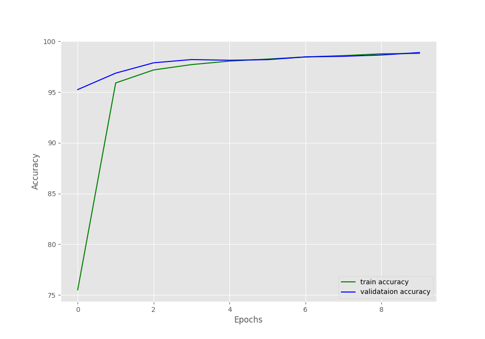
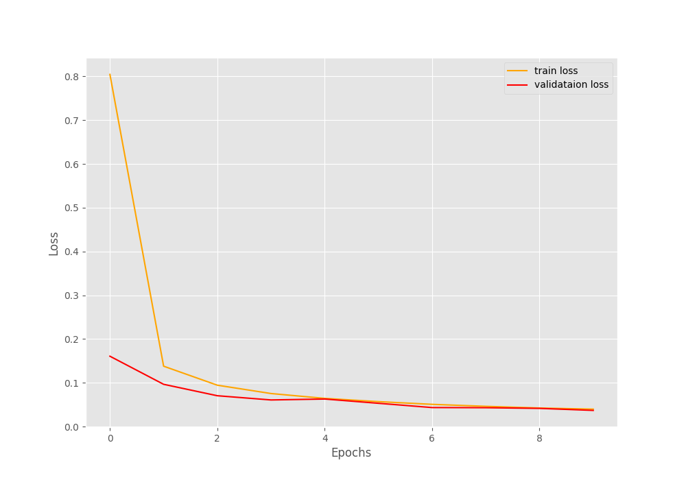
At the end of 30 epochs, the validation loss is 0.029, and validation accuracy is 99.14%. This seems pretty good. Hopefully, the neural network has learned the features of the dataset well.

Visualizing Class Activation Map using Trained Model

We have trained our model on the MNIST dataset by now. The next step is to load this trained model, feed it some new unseen digit images and visualize the class activation maps.

We will reuse most of the code from this post with little tweaks. If you are new to class activation map in PyTorch, then please go through that post. We will not dive into much of the details of the code in this post.

All the code here will go into the cam.py script.

The following code block contains all the import statements.

import numpy as np
import cv2
import torch
import glob as glob

from torchvision import transforms
from torch.nn import functional as F
from torch import topk
from model import Net

We will need the Net class to initialize the model again before loading the trained weights.

The next code block initializes the computation device and the model. It also loads the trained weights from the disk into the model.

# define computation device
device = ('cuda' if torch.cuda.is_available() else 'cpu')
# initialize model, switch to eval model, load trained weights
model = Net()
model = model.eval()
model.load_state_dict(torch.load('model.pth'))

Function to Generate and Return Class Activation Map

To get the class activation map for a particular image, we need the convolutional features, the softmax weights, and the class index for the most confident prediction. We will get the top 1 prediction using the topk function.

# https://github.com/zhoubolei/CAM/blob/master/pytorch_CAM.py
def returnCAM(feature_conv, weight_softmax, class_idx):
    # generate the class activation maps upsample to 256x256
    size_upsample = (256, 256)
    bz, nc, h, w = feature_conv.shape
    output_cam = []
    for idx in class_idx:
        cam = weight_softmax[idx].dot(feature_conv.reshape((nc, h*w)))
        cam = cam.reshape(h, w)
        cam = cam - np.min(cam)
        cam_img = cam / np.max(cam)
        cam_img = np.uint8(255 * cam_img)
        output_cam.append(cv2.resize(cam_img, size_upsample))
    return output_cam

The returnCAM() function accepts the feature_conv, weight_softmax, and class_idx as parameters and returns the final output class activation map.

The next function is a simple one to show the final image with the class activation map overlayed on top of it.

def show_cam(CAMs, width, height, orig_image, class_idx, save_name):
    for i, cam in enumerate(CAMs):
        heatmap = cv2.applyColorMap(cv2.resize(cam,(width, height)), cv2.COLORMAP_JET)
        result = heatmap * 0.5 + orig_image * 0.5
        # put class label text on the result
        cv2.putText(result, str(int(class_idx[i])), (20, 40), 
                    cv2.FONT_HERSHEY_SIMPLEX, 1, (0, 255, 0), 2)
        cv2.imshow('CAM', result/255.)
        cv2.waitKey(0)
        cv2.imwrite(f"outputs/CAM_{save_name}.jpg", result)

In the show_cam() function, we are:

• Generating a heatmap for the class activation map using the COLORMAP_JET of OpenCV.
• On line 33, we are blending both, the heatmap and the original image.
• Then we are putting the class text on top of the final image, visualizing it, and saving it to disk.

Forward Hook to Get the Convolutional Features

If you remember our model has a conv feature extractor. We will use a function that will attach a forward hook and extract all the convolutional layer’s features. Those are the highlighted layers in the following network architecture that we have.

Net(
  (conv): Sequential(
    (0): Conv2d(1, 16, kernel_size=(5, 5), stride=(1, 1))
    (1): ReLU()
    (2): MaxPool2d(kernel_size=2, stride=2, padding=0, dilation=1, ceil_mode=False)
    (3): Conv2d(16, 32, kernel_size=(4, 4), stride=(1, 1))
    (4): ReLU()
    (5): MaxPool2d(kernel_size=2, stride=2, padding=0, dilation=1, ceil_mode=False)
  )
  (linear): Sequential(
    (0): Linear(in_features=512, out_features=32, bias=True)
    (1): ReLU()
    (2): Linear(in_features=32, out_features=10, bias=True)
  )
)

# hook the feature extractor
# https://github.com/zhoubolei/CAM/blob/master/pytorch_CAM.py
features_blobs = []
def hook_feature(module, input, output):
    features_blobs.append(output.data.cpu().numpy())
model._modules.get('conv').register_forward_hook(hook_feature)
# get the softmax weight
params = list(model.parameters())
weight_softmax = np.squeeze(params[-2].data.numpy())

On line 45, we are registering a forward hook for the conv module of the model that will extract the features from the two convolutional layers.

Define the Transform and Perform the Forward Pass

Next, we define the image transforms that we need.

# define the transforms, resize => tensor => normalize
transform = transforms.Compose(
    [transforms.ToPILImage(),
     transforms.Resize((28, 28)),
     transforms.ToTensor(),
     transforms.Normalize(
        mean=[0.5],
        std=[0.5])
    ])

The test images that we have are custom made and more than 200×200 in dimensions. But our model accepts inputs of 28×28. So, we are resizing the images to that dimension.

Now, we will run a for loop over all the image paths and do the forward pass through the model.

# run for all the images in the `input` folder
for image_path in glob.glob('input/*'):
    # read the image
    image = cv2.imread(image_path)
    orig_image = image.copy()
    image = cv2.cvtColor(image, cv2.COLOR_BGR2GRAY)
    image = np.expand_dims(image, axis=2)
    height, width, _ = orig_image.shape
    # apply the image transforms
    image_tensor = transform(image)
    # add batch dimension
    image_tensor = image_tensor.unsqueeze(0)
    # forward pass through model
    outputs = model(image_tensor)
    # get the softmax probabilities
    probs = F.softmax(outputs).data.squeeze()
    # get the class indices of top k probabilities
    class_idx = topk(probs, 1)[1].int()
    
    # generate class activation mapping for the top1 prediction
    CAMs = returnCAM(features_blobs[0], weight_softmax, class_idx)
    # file name to save the resulting CAM image with
    save_name = f"{image_path.split('/')[-1].split('.')[0]}"
    # show and save the results
    show_cam(CAMs, width, height, orig_image, class_idx, save_name)

• After reading the image we are keeping an original copy for final visualizations (line 62).
• Remember that our model can only handle grayscale images. So we are converting the image to grayscale format appending a single channel color dimension at the end (lines 63 and 64).
• Line 71 does the forward pass through the model.
• On line 78, we call the returnCAM() function that gives us the class activation map.
• Finally, we call the show_cam() function on line 82.

This completes all the code we need for visualizing class activation map using PyTorch.

Execute cam.py

Now, let’s execute the cam.py script. This will show all the images one by one and we need to keep on pressing a key on the keyboard to see the next image.

python cam.py

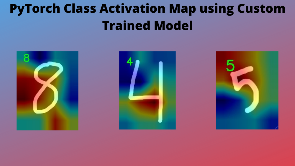
Except for two, the model predicts all other images correctly. Let’s see what the model predicted correctly and why it thought so for a few of the correct predictions.

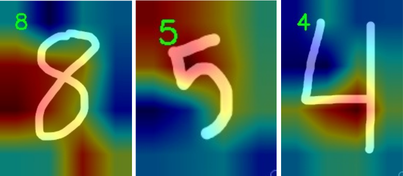
For digit eight, the model is mostly looking at the rounded corners and the middle part where the lines cross. This seems pretty good. For digit 5, the model is figuring out by looking at the top portion. And for the letter four, the model predicts so by focusing on the part where the two lines cross almost perpendicularly. These seem like good reasons for predictions.

We have two wrong predictions as well.

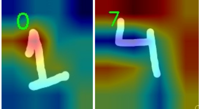
The model is predicting the digit as 7 instead of four. It looks like it is almost completely missing out on the long straight line. This might be because after the two lines cross perpendicularly, the long line does not extend much to the top. And therefore, the model thought it might be a 7. For digit 1, the model is almost entirely focusing on the top part and a bit on the middle. That leads to the prediction as 0. This does not seem very clear why the model might think so.

A Few Takeaways and Further Experiments

• Using class activation maps, we can interpret why a model predicted a certain class. Although it might not be clear in a few of the cases, still we can get good insights most of the time.
• For further experiments, try removing the pooling layers. This will lead to higher resololution activation maps. Those will be more localized and give even better insights. You will need to change the number of neurons in the first linear layer after removing the pooling layers. If you find the results interesting, do post in the comment section for others to see.

Summary and Conclusion

In this tutorial, you learned how to interpret model predictions by generating class activation on a custom trained model. We trained a very simple model on the MNIST dataset and this can be used as a stepping stone for more complex projects. I hope that you learned something new from this tutorial.

If you have any doubts, thoughts, or suggestions, then please leave them in the comment section. I will surely address them.

You can contact me using the Contact section. You can also find me on LinkedIn, and Twitter.