More than Real-Time FPS using SqueezeNet for Image Classification in PyTorch

In this tutorial, you will learn how to use a pre-trained SqueezeNet model in PyTorch for Image Classification.

You must have used a number of deep learning models for image classification. We often use ImageNet pre-trained models like ResNets, VGG nets, DenseNets for image classification on more than 1000 classes. Models like MobileNets are pretty fast, giving real-time speed. But there are a few models like SqueezeNet which are even faster than MobileNets.

Although generally, we do not use image classification models for inferencing on videos, still we can do that. If we can find a video that contains a single class for most of the frames, then we can run inference using them and even calculate the FPS. And for images, we can always calculate the forward pass time easily. This is exactly what we are going to do in this tutorial.

We will cover the following topics in this tutorial:

• First of all, we will use a pre-trained SqueezeNet model for both image and video classification in PyTorch.
• For the inference on images, we will calculate the time taken from the forward pass through the SqueezeNet model.
• For the inference on videos, we will calculate the FPS. To get some reasoable results, we will run inference on videos mostly containing a single class.
• Along with that, we will also run inference on both CPU and GPU and compare the FPS and forward pass time.
• Finally, we will end the tutorial with the key takeaways and the summary & conclusion.

Note: We will not go through the details of the SqueezeNet model in this tutorial. Rather, we will focus on carrying out inference using the pre-trained model. We will cover the complete details of the SqueezeNet model in future posts and tutorials.

Directory Structure

Let’s take a look at the directory structure for this tutorial. We will set this up and then move towards the coding part.

├── input
│   ├── image_1.jpg
│   ├── image_2.jpg
│   ├── video_1.mp4
│   └── video_2.mp4
├── outputs
│   ├── image_1.jpg
│   ...
│   └── video_1_cuda.mp4
├── classify_image.py
├── classify_video.py
├── imagenet_classes.txt
└── utils.py

• The input folder contains the images and videos that we will use for inference.
• The outputs folder will containt the corresponding inference results.
• We have three Python scripts:
  • classify_image.py contians the code to carry out image classification using SqueezeNet in PyTorch.
  • classify_video.py contains the code to carry out classification on vidoes using SqueezeNet in PyTorch.
  • And utils.py contains the helper functions. We will go through these in detail in later part of the post.
• Finally, we have the imagenet_classes.txt which contains the 1000 class names from the ImageNet dataset. We will use this to show the class text after forward passing the image through the model and mapping the prediction label to the names in this file.

You will find all the files and folders for this tutorial when downloading the related zip file and extracting it.

The PyTorch Version

Please note that all the code in this tutorial uses PyTorch 1.9.0. If you do not have PyTorch installed in your system yet, you can very easily do that from the official website.

Image and Video Classification using SqueezeNet in PyTorch

Let’s start with the coding part of the tutorial without any further delay. We will:

• First write the helper functions in the utils.py script.
• Then move on to the classify_images.py script, write the code and execute to see the outputs on both CPU and GPU.
• Finally, will write the code for classify_videos.py script and carry inference on videos.

The Utility Script

We will write three helper functions which will be used for both, inferencing on images and videos as well.

All the code here will go into the utils.py script.

Let’s start with the import statements and the first function.

import torchvision.models as models

from torchvision import transforms

def load_model():
    """
    Load the pre-trained SqueezeNet model.
    """
    model = models.squeezenet1_0(pretrained=True)
    model.eval()
    return model

• We need to the models module from torchvision to download the pre-trained SqueezeNet model.
• We will apply the image transforms using transforms.

The above code block also contains the load_model() function which loads the pre-trained SqueezeNet model. Note that we are loading the squeezenet1_0 model. Going through the official PyTorch script states that this is the larger of the two models as described in the SqueezeNet paper. There is also the squeezenet1_1 model which requires 2.4x less computation and has a bit fewer parameters. But the accuracy remains the same according to the official script. In this tutorial, we will stick with the former model.

Next, the preprocessing function.

def preprocess():
    """
    Define the transform for the input image/frames.
    Resize, crop, convert to tensor, and apply ImageNet normalization stats.
    """
    transform =  transforms.Compose([
        transforms.ToPILImage(),
        transforms.Resize(256),
        transforms.CenterCrop(224),
        transforms.ToTensor(),
        transforms.Normalize(mean=[0.485, 0.456, 0.406], 
                             std=[0.229, 0.224, 0.225]),])
    return transform

The preprocess() function defines the image transforms.

• We resize the image to 256×256 dimensions.
• Then apply center cropping to reduce the size further to 224×224.
• Convert the images to tensors and apply the ImageNet normalization statistics.

The final helper function is to load the ImageNet class names.

def read_classes():
    """
    Load the ImageNet class names.
    """
    with open("imagenet_classes.txt", "r") as f:
        categories = [s.strip() for s in f.readlines()]
    return categories

The read_classes() function returns the class names (categories) after reading and stripping the class names by new lines from the imagenet_classes.txt file.

Image Classification using SqueezeNet in PyTorch

In this section, we will carry out image classification using SqueezeNet in PyTorch. As we have already written the helper functions, the coding will become much simpler.

The code in this section will go into the classify_image.py script.

The following are the imports that we need for image classification.

import torch
import cv2
import argparse
import time

from utils import load_model, preprocess, read_classes

We will need the time module to calculate the time taken for each image for the forward pass. We are also importing all the functions from the utils script.

Now, let’s construct the argument parser.

# construct the argumet parser to parse the command line arguments
parser = argparse.ArgumentParser()
parser.add_argument('-i', '--input', default='input/image_1.jpg', 
                    help='path to the input image')
parser.add_argument('-d', '--device', default='cpu', 
                    help='computation device to use', 
                    choices=['cpu', 'cuda'])
args = vars(parser.parse_args())

• The --input flag is for passing the path to the input image while executing the script.
• And --device flag is for passing the computation device. We can pass either the cpu or cuda as the computation device.

Initialize the Device, Model, Class Names, And Transforms

The next block of code initializes the computation device, the ImageNet class names, the model, and the image transforms.

# set the computation device
DEVICE = args['device']
# initialize the model
model = load_model()
# load the ImageNet class names
categories = read_classes()
# initialize the image transforms
transform = preprocess()

print(f"Computation device: {DEVICE}")

We have already imported the functions defined in the utils module. We just call the functions in the above code block. The categories contains the class names and transform contains the image transforms.

Read the Image and Forward Pass Through the Model

The next code block contains the final set of code. It reads the image and carries out the forward pass through the model.

image = cv2.imread(args['input'])
rgb_image = cv2.cvtColor(image, cv2.COLOR_BGR2RGB)
# apply transforms to the input image
input_tensor = transform(image)
# add the batch dimensionsion
input_batch = input_tensor.unsqueeze(0)

# move the input tensor and model to the computation device
input_batch = input_batch.to(DEVICE)
model.to(DEVICE)

with torch.no_grad():
    start_time = time.time()
    output = model(input_batch)
    end_time = time.time()

# get the softmax probabilities
probabilities = torch.nn.functional.softmax(output[0], dim=0)

# check the top 5 categories that are predicted
top5_prob, top5_catid = torch.topk(probabilities, 5)
for i in range(top5_prob.size(0)):
    cv2.putText(image, f"{top5_prob[i].item()*100:.3f}%", (15, (i+1)*30), cv2.FONT_HERSHEY_SIMPLEX,
                1, (0, 255, 0), 2, cv2.LINE_AA)
    cv2.putText(image, f"{categories[top5_catid[i]]}", (160, (i+1)*30), cv2.FONT_HERSHEY_SIMPLEX,
                1, (0, 255, 0), 2, cv2.LINE_AA)
    print(categories[top5_catid[i]], top5_prob[i].item())

cv2.imshow('Result', image)
cv2.waitKey(0)

# define the outfile file name
save_name = f"outputs/{args['input'].split('/')[-1].split('.')[0]}_{DEVICE}.jpg"
cv2.imwrite(save_name, image)
print(f"Forward pass time: {(end_time-start_time):.3f} seconds")

• We are reading the image and converting the image to RGB color format.
• Then we are applying the image transforms and adding a batch dimension.
• On lines 33 and 34, we are loading the input tensor and model on to the computation device.
• From line 36, we are starting the forward pass block. The forward pass happens within the with torch.no_grad() block so that the gradients do not get calculated.
• Then we get the softmax probabilities on line 42.
• Line 45 extracts the top 5 probility scores and category indices from the probabilities.
• The next for loop puts the class label text and probability scores for the top 5 predictions on the image. We print the results as well.
• Then we show the image on screen and save the resulting image to disk. The resulting save_name string also contains the DEVICE name so that we can differentiate between different runs of the script.
• Finally, we print the forward pass time.

Execute classify_image.py Script

We have completed the script for classifying images using SqueezeNet. Let’s execute the classify_image.py script. Make sure to open your command line/terminal in the current working directory (where the Python Scripts are present).

All the results shown here are carried out on a laptop with an 8th Gen i7 CPU, 16 GB of RAM, and a 6GB GTX 1060 GPU.

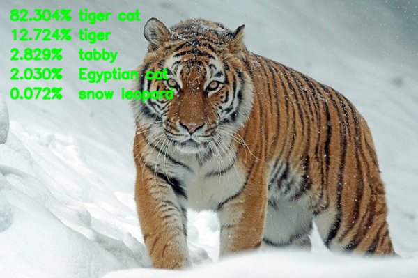
Classifying image_1.jpg using CPU as the computation device.

python classify_image.py -d cpu -i input/image_1.jpg

The following are the outputs.

Eskimo dog 0.5426698923110962
Siberian husky 0.3717397153377533
malamute 0.049058761447668076
Cardigan 0.014761386439204216
toy terrier 0.009008544497191906
Forward pass time: 0.026 seconds

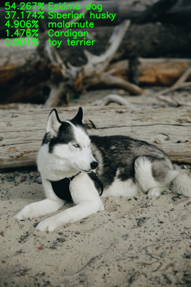
The model predicted Eskimo dog with the highest confidence which is the correct prediction. And it took only 0.026 seconds for the forward pass.

Let’s execute using the GPU as the computation device.

python classify_image.py -d cuda -i input/image_1.jpg

Eskimo dog 0.542668879032135
Siberian husky 0.3717404007911682
malamute 0.04905867204070091
Cardigan 0.014761414378881454
toy terrier 0.009008579887449741
Forward pass time: 0.108 seconds

Interestingly it took 0.108 seconds for the forward pass which is more than the CPU computation time.

Let’s check with another image before making any conclusions.

python classify_image.py -d cpu -i input/image_2.jpg

sports car 0.6201938986778259
convertible 0.15191926062107086
racer 0.08226030319929123
cab 0.06592991948127747
grille 0.024620428681373596
Forward pass time: 0.020 seconds

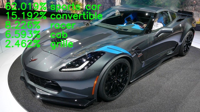
This time also the highest confidence prediction is correct, that is a sports car and it took only 0.020 seconds for the forward pass.

What about the GPU inference time?

python classify_image.py -d cpu -i input/image_2.jpg

sports car 0.6201937794685364
convertible 0.15191952884197235
racer 0.0822601318359375
cab 0.06592990458011627
grille 0.024620281532406807
Forward pass time: 0.115 seconds

Again, the forward pass time is more than that of the CPU.

This might be because GPUs perform well when utilized to their full capacity so using higher batch sizes might help. Higher batch sizes allow the usage of almost all the cores of the GPU which leads to more efficient and faster computation. As we are passing only one image here, therefore, we are not able to use the GPU to the fullest.

Most probably, we will be able to get much higher FPS when inferencing using GPU when passing one frame after the other in the case of video streams. Let’s check that out in the next section.

Video Classification using SqueezeNet in PyTorch

In this section, we will start writing the code to classify videos using SqueezeNet in PyTorch. All the code here will go into the classify_video.py file.

The code till preparing the image transforms is going to remain the same as was when classifying images. So, let’s get done with that first.

import torch
import cv2
import time
import argparse

from utils import load_model, preprocess, read_classes

# construct the argumet parser to parse the command line arguments
parser = argparse.ArgumentParser()
parser.add_argument('-i', '--input', default='input/video_1.mp4', 
                    help='path to the input video')
parser.add_argument('-d', '--device', default='cpu', 
                    help='computation device to use', 
                    choices=['cpu', 'cuda'])
args = vars(parser.parse_args())

# set the computation device
DEVICE = args['device']
# initialize the model
model = load_model()
# load the ImageNet class names
categories = read_classes()
# initialize the image transforms
transform = preprocess()

print(f"Computation device: {DEVICE}")

Only this time, for the --input flag, instead of an image, we will provide the path to a video file.

Reading the Video File

Let’s read the video file now and set up the VideoWriter object as well to save the resulting video file.

cap = cv2.VideoCapture(args['input'])
# get the frame width and height
frame_width = int(cap.get(3))
frame_height = int(cap.get(4))
# define the outfile file name
save_name = f"{args['input'].split('/')[-1].split('.')[0]}_{DEVICE}"
# define codec and create VideoWriter object 
out = cv2.VideoWriter(f"outputs/{save_name}.mp4", 
                      cv2.VideoWriter_fourcc(*'mp4v'), 30, 
                      (frame_width, frame_height))
# to count the total number of frames iterated through
frame_count = 0
# to keep adding the frames' FPS
total_fps = 0

We need the video frames’ width and height to initialize the VideoWriter object for saving the output video file. We are also declaring two more variables, frame_count and total_fps. These are to count to the total number of frames iterated through and the counting the total Frames Per Second (FPS) till the end.

Iterate Over the Video Frames

Now, it’s time to iterate over the video frames and carry out the prediction for each frame. A simple while loop will work effectively here.

while(cap.isOpened()):
    # capture each frame of the video
    ret, frame = cap.read()
    if ret:
        rgb_frame = cv2.cvtColor(frame, cv2.COLOR_BGR2RGB)
        # apply transforms to the input image
        input_tensor = transform(rgb_frame)
        # add the batch dimensionsion
        input_batch = input_tensor.unsqueeze(0) 

        # move the input tensor and model to the computation device
        input_batch = input_batch.to(DEVICE)
        model.to(DEVICE)

        with torch.no_grad():
            start_time = time.time()
            output = model(input_batch)
            end_time = time.time()

        # get the softmax probabilities
        probabilities = torch.nn.functional.softmax(output[0], dim=0)
        # get the top 1 prediction
        top1_prob, top1_catid = torch.topk(probabilities, 1)

        # get the current fps
        fps = 1 / (end_time - start_time)
        # add `fps` to `total_fps`
        total_fps += fps
        # increment frame count
        frame_count += 1
        cv2.putText(frame, f"{fps:.3f} FPS", (15, 30), cv2.FONT_HERSHEY_SIMPLEX,
                        1, (0, 255, 0), 2)
        cv2.putText(frame, f"{categories[top1_catid[0]]}", (15, 60), cv2.FONT_HERSHEY_SIMPLEX,
                        1, (0, 255, 0), 2)
        cv2.imshow('Result', frame)
        out.write(frame)
        if cv2.waitKey(1) & 0xFF == ord('q'):
            break
    else:
        break
    
# release VideoCapture()
cap.release()
# close all frames and video windows
cv2.destroyAllWindows()
# calculate and print the average FPS
avg_fps = total_fps / frame_count
print(f"Average FPS: {avg_fps:.3f}")

Until we have frames present in the video file:

• We capture the frame and convert it to RGB color format to pass through the model (line 45).
• Then we apply the transforms, add the batch dimension, and load the model and frame on to the computation device.
• Starting from line 55, we carry out the prediction.
• This time, instead of top 5 predictions, we get the top 1 prediction only.
• Then we calculate the FPS and put the class label and FPS texts on the current video frame (lines 65 to 74).
• Before ending the loop, we show the resulting frame on the screen, and save it to disk as well.

Finally, we release the VideoCapture object, destroy all OpenCV windows and print the average FPS value.

Execute classify_video.py Script

Let’s execute the classify_video.py script and check out the FPS on both CPU and GPU. We have two videos in the input folder, but let’s carry out inference on one of them here.

Starting off with the GPU inference.

python classify_video.py -d cuda -i input/video_1.mp4

The following is the output on the terminal.

Computation device: cuda
Average FPS: 528.082

We are getting an astounding 528 FPS on average! To be completely fair, that’s a lot. The predictions remain as sports car for most of the frames, but we can see it fluctuating between convertible and bullet train as well. Obviously, when a model gives this much FPS, the predictions are bound to take a hit. And that’s exactly what is happening here.

Just to have an idea, let’s check out the average FPS when using CPU as the computation device.

python classify_video.py -d cpu -i input/video_1.mp4

Computation device: cpu
Average FPS: 66.704

We are getting 66.7 FPS, which is still a lot. That’s a really good number for CPU as the computation device.

A Few Takeaways

• We saw how we can use the SqueezeNet model to carry out inference with GPU and get really high FPS.
• Even with CPU as the computation device, the average FPS was more than 60.
• This shows that the SqueezeNet model can be used as a backbone to build very fast object detection models which can give real-time FPS on mobile devices easily.

Summary and Conclusion

You learned how to carry out image and video classification using SqueezeNet in PyTorch in this tutorial. We also got to know the high FPS that we can get while using GPU as the computation device. I hope that you learned something new from this tutorial.

If you have any doubts, thoughts, or suggestions, then please leave them in the comment section. I will surely address them.

You can contact me using the Contact section. You can also find me on LinkedIn, and Twitter.