PyTorch ImageFolder for Training CNN Models

In this tutorial, you will learn how to use the PyTorch ImageFolder class for easily training CNN models.

Why This Tutorial?

Deep learning image datasets do not always have a proper structure. Sometimes images are just present in their respective folders where the folder name corresponds to the class they belong to. In many such cases, we as developers, tend to write extra Python code to create CSV files where the image names map to the folders they are present in along with a column representing the corresponding class.

This might look something like the following.

Image ID	Path	Class
image_1	../input/folder1/image_1.jpg	class_1
image_2	../input/folder2/image_2.jpg	class_2

But we might not have this convenience always. In such cases, we write the extra code to create such a file that will help us while reading the images and assign the correct labels to the corresponding images while training.

And that’s where the PyTorch ImageFolder class comes into play.

So, what all are we covering in this tutorial?

• We will learn how to use the PyTorch ImageFolder class for effectively training CNN models.
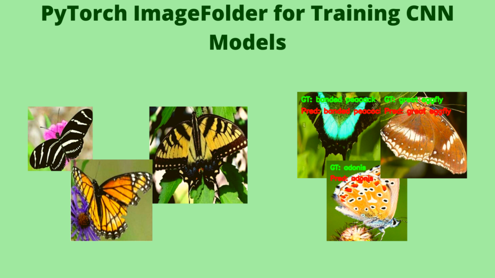
• Along with that, we will also tackle a very interesting problem. We will use the ImageFolder class to prepare the dataset for classifying butterfly images. We will use this dataset from Kaggle which contains images belonging to 50 different species of butterflies.
• After training the model, we will also use the saved model for inference on new test images.

So, along with learning about the PyTorch ImageFolder, we will also tackle a very interesting problem using a custom neural network model. I hope that you are excited to follow along with this tutorial.

PyTorch ImageFolder Class

Let’s go over the PyTorch ImageFolder class in brief. It’s a fairly easy concept to grasp.

The ImageFolder class is a part of the torchvision library’s datasets module. We can easily access it using the following syntax:

torchvision.datasets.ImageFolder

This class helps us to easily create PyTorch training and validation datasets without writing custom classes. Then we can use these datasets to create our iterable data loaders.

Basically, the ImageFolder class inherits from the DatasetFolder class. So, we can override the classes to create custom datasets as well.

But how should our image dataset folder be structured to use it? Frankly, this is the best part of using this class. The image datasets folder should be of the following structure:

├── train
│   ├── class1
|      ├── 1.jpg
│      ├── 2.jpg
│   ├── class2
|      ├── 1.jpg
│      ├── 2.jpg
├── valid
│   ├── class1
|      ├── 1.jpg
│      ├── 2.jpg
│   ├── class2
|      ├── 1.jpg
│      ├── 2.jpg

If you observe closely, this is how many of the image datasets for deep learning are structured. This means that we can easily use the PyTorch ImageFolder for training CNN models.

So, what should be the actual syntax to create the training and validation datasets? Well, quite straightforward.

train_dataset = torchvision.datasets.ImageFolder(root='train')

valid_dataset = torchvision.datasets.ImageFolder(root='valid')

Yes, we just need to provide the path to the root train and valid folders. All the other things will be taken care of by the ImageFolder class.

Please note that the train and valid folders can have other names as well. I have just kept these names for illustration here. Also, many of the image datasets for deep learning actually are separated by such names. So, it is most intuitive to learn it this way as well.

Next, we can very easily create training and validation data loaders.

train_loader = DataLoader(train_dataset, ...)

valid_loader = DataLoader(valid_dataset, ...)

Next up, let’s check the dataset that we will use in this tutorial and its directory structure.

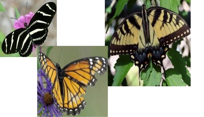
The Butterfly Image Classification Dataset

To know the usefulness of PyTorch ImageFolder for the effective training of CNN models, we will use a dataset that is in the required format.

The Butterfly Image Classification dataset from Kaggle contains 4955 images for training, 250 images for validation, and 250 images for testing. And all the images are 224×224 dimensional RGB images (having 3 color channels).

Each of the above splits has 50 subdirectories which act as the classes for the images. Let’s take a look at the structure.

├── butterflies
│   ├── test
│   │   ├── adonis
│   │   │   ├── 1.jpg
│   │   ...
│   │   └── zebra long wing
│   │       ├── 1.jpg
│   │       ...
│   ├── train
│   │   ├── adonis [96 entries exceeds filelimit, not opening dir]
│   │   ...
│   │   └── zebra long wing [108 entries exceeds filelimit, not opening dir]
│   ├── valid
│   │   ├── adonis
│   │   │   ├── 1.jpg
│   │   ...
│   │   └── zebra long wing
│   │       ├── 1.jpg
│   │       ...
├── butterflies_rev2
│   ├── images to predict
│   │   ├── 06.jpg
│   │   ...
│   ├── single image to predict
│   │   └── 06.jpg
│   ├── test
│   │   ├── adonis
│   │   │   ├── 1.jpg
|   |   |   ...
│   ├── train
│   │   ├── adonis [96 entries exceeds filelimit, not opening dir]
│   │   ...
│   │   └── zebra long wing [108 entries exceeds filelimit, not opening dir]
│   ├── valid
│   │   ├── adonis
│   │   ...
│   │   └── zebra long wing
│   │       ├── 1.jpg
│   │       ...
│   ├── butterflies.csv
│   ├── class_dict.csv

The above structure might seem a bit confusing at first. For that reason, I have highlighted the lines we need to focus on.

So, all the data we need are present in the butterflies_rev2 folder. It has the train and valid folder that we will use for creating the training and validation datasets respectively. The test folder also has a similar structure with 50 subdirectories. But we will use the images from that for inference after the training completes. For now, you can safely ignore any other folder or CSV file that comes with the dataset. We will not need those. Our ImageFolder class will be able to handle everything from the folders only.

Just one more thing. Before moving further, be sure to download the dataset from Kaggle. In the next section, we will see how the dataset should be arranged after extracting it.

Directory Strucutre

The following is the directory structure that we will use for this project.

├── input
│   ├── butterflies
│   ├── butterflies_rev2
├── outputs
│   ├── accuracy.png
│   ...
├── datasets.py
├── inference.py
├── model.py
├── train.py
└── utils.py

• The input folder will contain the Butterfly Image Classification dataset in the format that you see in the above block. Make sure that after extracting the content you too have the same structure so that you need not change the path in the Python script.
• The outputs folder will contain all the output images and the trained model that will be generated as a result of training and inference.
• Then we have five Python (.py) files. We will get into the details of these while writing the code in them.

PyTorch Version

The code in this tutorial has been run and tested on PyTorch 1.9.0. Having a slightly older version like 1.8.1 should not cause any issues as well. But it is always better to have the latest stable version.

PyTorch ImageFolder for Training CNN Models

From this section onward, we will start with the coding part of this tutorial.

We will start by writing a few helper functions.

Helper Functions

We will write two helper functions. These will help us save the trained model and the accuracy & loss plots after the training completes.

All the code in here will go into the utils.py Python file.

The following code block contains all the import statements and the first helper function.

import torch
import matplotlib
import matplotlib.pyplot as plt

matplotlib.style.use('ggplot')


def save_model(epochs, model, optimizer, criterion):
    """
    Function to save the trained model to disk.
    """
    torch.save({
                'epoch': epochs,
                'model_state_dict': model.state_dict(),
                'optimizer_state_dict': optimizer.state_dict(),
                'loss': criterion,
                }, 'outputs/model.pth')

The save_model() function in the above code block accepts the epochs, model, optimizer, and the criterion as parameters. We will use the torch.save() function to save the model state dictionary and optimizer state dictionary as well. If we want, we can easily resume training as well.

The next function is for saving the loss and accuracy plots after the training completes.

def save_plots(train_acc, valid_acc, train_loss, valid_loss):
    """
    Function to save the loss and accuracy plots to disk.
    """
    # accuracy plots
    plt.figure(figsize=(10, 7))
    plt.plot(
        train_acc, color='green', linestyle='-', 
        label='train accuracy'
    )
    plt.plot(
        valid_acc, color='blue', linestyle='-', 
        label='validataion accuracy'
    )
    plt.xlabel('Epochs')
    plt.ylabel('Accuracy')
    plt.legend()
    plt.savefig('outputs/accuracy.png')
    
    # loss plots
    plt.figure(figsize=(10, 7))
    plt.plot(
        train_loss, color='orange', linestyle='-', 
        label='train loss'
    )
    plt.plot(
        valid_loss, color='red', linestyle='-', 
        label='validataion loss'
    )
    plt.xlabel('Epochs')
    plt.ylabel('Loss')
    plt.legend()
    plt.savefig('outputs/loss.png')

The train_acc, valid_acc, train_loss, and valid_loss are lists containing the respective accuracy and loss values for each epoch. We use matplotlib to save the graphs to disk.

Preparing the Dataset and Data Loaders

Now, we will carry out one of the most important parts of this tutorial. We will prepare the dataset and data loaders that we need for training.

The code in this section will go into the datasets.py file.

The following code block contains the import statements and the batch size.

import torchvision.transforms as transforms
import torchvision.datasets as datasets

from torch.utils.data import DataLoader

# batch size
BATCH_SIZE = 64

We are using a batch size of 64. Along with the model that we will build, the image size that we will use, and this batch size, the VRAM usage is going to be somewhere around 3.3 GB. If you face OOM (Out Of Memory) error when running the code on your own machine, try using a batch size of 32 or 16.

Next, let’s define the training and validation transforms.

# the training transforms
train_transform = transforms.Compose([
    transforms.Resize((224, 224)),
    transforms.RandomHorizontalFlip(p=0.5),
    transforms.RandomVerticalFlip(p=0.5),
    transforms.GaussianBlur(kernel_size=(5, 9), sigma=(0.1, 5)),
    transforms.RandomRotation(degrees=(30, 70)),
    transforms.ToTensor(),
    transforms.Normalize(
        mean=[0.5, 0.5, 0.5],
        std=[0.5, 0.5, 0.5]
    )
])
# the validation transforms
valid_transform = transforms.Compose([
    transforms.Resize((224, 224)),
    transforms.ToTensor(),
    transforms.Normalize(
        mean=[0.5, 0.5, 0.5],
        std=[0.5, 0.5, 0.5]
    )
])

For the train_transform we are:

• Resizing the images to 224×224 dimensions. All the images are by default 224×224 dimensional. This resizing is just to ensure that we do not face any unseen errors during training.
• For the augmentations we are applying RandomHorizontalFlip, RandomVerticalFlip, GaussianBlur, and RandomRotation. From experiments, I found that without augmentations, the model was overfitting very soon.
• Finally, we are converting the images to tensors and normalizing them.

For the valid_transforms, we are just resizing, converting to tensors, and normalizing the images.

Now, we will prepare the datasets and data loaders. This is where the ImageFolder class comes into play.

# training dataset
train_dataset = datasets.ImageFolder(
    root='input/butterflies_rev2/train',
    transform=train_transform
)
# validation dataset
valid_dataset = datasets.ImageFolder(
    root='input/butterflies_rev2/valid',
    transform=valid_transform
)
# training data loaders
train_loader = DataLoader(
    train_dataset, batch_size=BATCH_SIZE, shuffle=True,
    num_workers=4, pin_memory=True
)
# validation data loaders
valid_loader = DataLoader(
    valid_dataset, batch_size=BATCH_SIZE, shuffle=False,
    num_workers=4, pin_memory=True
)

First, we prepare the train_dataset and the valid_dataset using torchvision.datastes.ImageFolder. We provide the root path to the train and valid folders respectively and the ImageFolder class takes care of the rest. No custom class or no defining labels for images are needed. It’s really easy. Along with that, we apply the respective transforms as well.

Then using the above datasets, we prepare the train_loader and valid_loader. We are using num_workers=4. If you are on Windows and face BrokenPipe error, consider changing the num_workers value to 0.

We are done with preparing our dataset. This was obviously much simpler than writing our own custom dataset classes.

The Neural Network Model

We will prepare a very simple, custom neural network model. We will not use any pre-trained models. This is also a sort of experiment, checking out how high of an accuracy we can achieve with a custom model.

Let’s check out the network architecture code below. The code will go into the model.py file.

import torch.nn as nn
import torch.nn.functional as F

class CNNModel(nn.Module):
    def __init__(self):
        super(CNNModel, self).__init__()
        self.conv1 = nn.Conv2d(3, 32, 5)
        self.conv2 = nn.Conv2d(32, 64, 5)
        self.conv3 = nn.Conv2d(64, 128, 3)
        self.conv4 = nn.Conv2d(128, 256, 5)
        
        self.fc1 = nn.Linear(256, 50)
        
        self.pool = nn.MaxPool2d(2, 2)
        
    def forward(self, x):
        x = self.pool(F.relu(self.conv1(x)))
        x = self.pool(F.relu(self.conv2(x)))
        x = self.pool(F.relu(self.conv3(x)))
        x = self.pool(F.relu(self.conv4(x)))
        bs, _, _, _ = x.shape
        x = F.adaptive_avg_pool2d(x, 1).reshape(bs, -1)
        x = self.fc1(x)
        return x

It’s a pretty simple neural network actually.

• We have four convolutional layers. And each subsequent layer has double the number of out_channels than the previous one.
• Each of the convolutional layers is followed by ReLU activation and max-pool 2D.
• We just have one linear layer with 50 out_features which equals to the number of classes in the dataset.

The only thing to notice in the above neural network is the kernel size. The first two convolutional layers have 5×5 kernels, then the next one is 3×3, and the last one is again a 5×5 kernel.

The Training Script

We finally get down to write the training script which is the one that we will run from the command line/terminal.

The training code will go into the train.py script.

Let’s import all the libraries, modules, and construct the argument parser.

import torch
import argparse
import torch.nn as nn
import torch.optim as optim
import time

from tqdm.auto import tqdm

from model import CNNModel
from datasets import train_loader, valid_loader
from utils import save_model, save_plots

# construct the argument parser
parser = argparse.ArgumentParser()
parser.add_argument('-e', '--epochs', type=int, default=20,
    help='number of epochs to train our network for')
args = vars(parser.parse_args())

We are importing:

• The train_loader, valid_loader from the datasets module.
• The CNNModel from model module.
• And save_model, and save_plots functions from utils.

For the argument parser, we just have one flag to specify the number of epochs to train for.

Setting Learning Parameters and Model Initialization

We will set the learning parameters like the learning rate, the computation device, and initialize the model as well.

# learning_parameters 
lr = 1e-3
epochs = args['epochs']
device = ('cuda' if torch.cuda.is_available() else 'cpu')
print(f"Computation device: {device}\n")

model = CNNModel().to(device)
print(model)
# total parameters and trainable parameters
total_params = sum(p.numel() for p in model.parameters())
print(f"{total_params:,} total parameters.")
total_trainable_params = sum(
    p.numel() for p in model.parameters() if p.requires_grad)
print(f"{total_trainable_params:,} training parameters.")

# optimizer
optimizer = optim.Adam(model.parameters(), lr=lr)
# loss function
criterion = nn.CrossEntropyLoss()

We are printing the model architecture and the number of parameters. Along with that, we are also defining the Adam optimizer with a 0.001 learning rate and the Cross-Entropy loss function.

The Training and Validation Functions

The training and validation functions are going to be pretty simple. Let’s take a look.

# training
def train(model, trainloader, optimizer, criterion):
    model.train()
    print('Training')
    train_running_loss = 0.0
    train_running_correct = 0
    counter = 0
    for i, data in tqdm(enumerate(trainloader), total=len(trainloader)):
        counter += 1
        image, labels = data
        image = image.to(device)
        labels = labels.to(device)
        optimizer.zero_grad()
        # forward pass
        outputs = model(image)
        # calculate the loss
        loss = criterion(outputs, labels)
        train_running_loss += loss.item()
        # calculate the accuracy
        _, preds = torch.max(outputs.data, 1)
        train_running_correct += (preds == labels).sum().item()
        # backpropagation
        loss.backward()
        # update the optimizer parameters
        optimizer.step()
    
    # loss and accuracy for the complete epoch
    epoch_loss = train_running_loss / counter
    epoch_acc = 100. * (train_running_correct / len(trainloader.dataset))
    return epoch_loss, epoch_acc

# validation
def validate(model, testloader, criterion):
    model.eval()
    print('Validation')
    valid_running_loss = 0.0
    valid_running_correct = 0
    counter = 0
    with torch.no_grad():
        for i, data in tqdm(enumerate(testloader), total=len(testloader)):
            counter += 1
            
            image, labels = data
            image = image.to(device)
            labels = labels.to(device)
            # forward pass
            outputs = model(image)
            # calculate the loss
            loss = criterion(outputs, labels)
            valid_running_loss += loss.item()
            # calculate the accuracy
            _, preds = torch.max(outputs.data, 1)
            valid_running_correct += (preds == labels).sum().item()
        
    # loss and accuracy for the complete epoch
    epoch_loss = valid_running_loss / counter
    epoch_acc = 100. * (valid_running_correct / len(testloader.dataset))
    return epoch_loss, epoch_acc

The above train and validate functions contain pretty standard code for what we generally write in PyTorch for image classification. In both cases, we are returning the loss and accuracy values after each epoch.

The Training Loop

The last thing we need to start the training is the training loop. We will use a simple for loop iterating through the number of epochs that we provide while executing the script.

# lists to keep track of losses and accuracies
train_loss, valid_loss = [], []
train_acc, valid_acc = [], []
# start the training
for epoch in range(epochs):
    print(f"[INFO]: Epoch {epoch+1} of {epochs}")
    train_epoch_loss, train_epoch_acc = train(model, train_loader, 
                                              optimizer, criterion)
    valid_epoch_loss, valid_epoch_acc = validate(model, valid_loader,  
                                                 criterion)
    train_loss.append(train_epoch_loss)
    valid_loss.append(valid_epoch_loss)
    train_acc.append(train_epoch_acc)
    valid_acc.append(valid_epoch_acc)
    print(f"Training loss: {train_epoch_loss:.3f}, training acc: {train_epoch_acc:.3f}")
    print(f"Validation loss: {valid_epoch_loss:.3f}, validation acc: {valid_epoch_acc:.3f}")
    print('-'*50)
    time.sleep(5)
    
# save the trained model weights
save_model(epochs, model, optimizer, criterion)
# save the loss and accuracy plots
save_plots(train_acc, valid_acc, train_loss, valid_loss)
print('TRAINING COMPLETE')

• We have four lists in the above code block. The train_loss, valid_loss, train_acc, valid_acc will keep on storing the loss and accuracy values for each of the training and validation epochs.
• Inside the training loop, we are printing the loss and accuracy information after each epoch.
• After the training completes we are saving the final model and the accuracy and loss graphs also.

This is all we need for the training code.

Execute train.py Script

We are all set to execute the train.py script. Open your command line/terminal in the directory where the training script is present and execute the following command. We will train the neural network model for 45 epochs.

python train.py --epochs 45

The following is the truncated output from the terminal.

Computation device: cuda

CNNMOdel(
  (conv1): Conv2d(3, 32, kernel_size=(5, 5), stride=(1, 1))
  (conv2): Conv2d(32, 64, kernel_size=(5, 5), stride=(1, 1))
  (conv3): Conv2d(64, 128, kernel_size=(3, 3), stride=(1, 1))
  (conv4): Conv2d(128, 256, kernel_size=(5, 5), stride=(1, 1))
  (fc1): Linear(in_features=256, out_features=50, bias=True)
  (pool): MaxPool2d(kernel_size=2, stride=2, padding=0, dilation=1, ceil_mode=False)
)
959,858 total parameters.
959,858 training parameters.
[INFO]: Epoch 1 of 45
Training
100%|███████████████████████████████████████████| 78/78 [00:38<00:00,  2.02it/s]
Validation
100%|█████████████████████████████████████████████| 4/4 [00:00<00:00,  4.16it/s]
Training loss: 3.468, training acc: 7.790
Validation loss: 3.060, validation acc: 14.800
--------------------------------------------------
...
[INFO]: Epoch 45 of 45
Training
100%|███████████████████████████████████████████| 78/78 [00:36<00:00,  2.12it/s]
Validation
100%|█████████████████████████████████████████████| 4/4 [00:00<00:00,  5.19it/s]
Training loss: 0.381, training acc: 87.386
Validation loss: 0.942, validation acc: 76.400
--------------------
TRAINING COMPLETE

And the following are the loss and accuracy graphs.

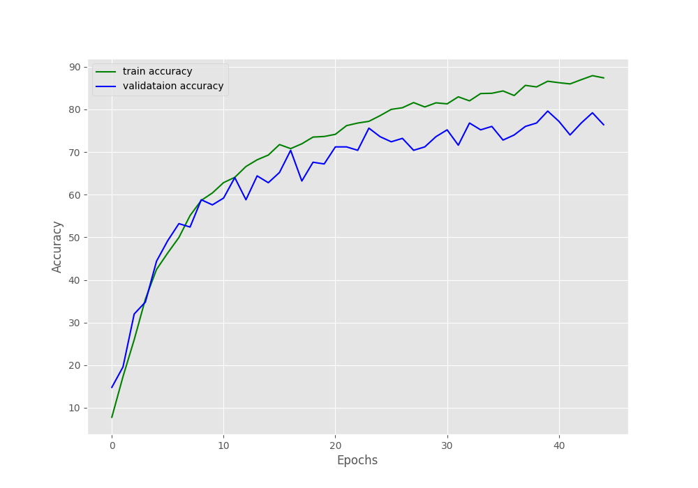
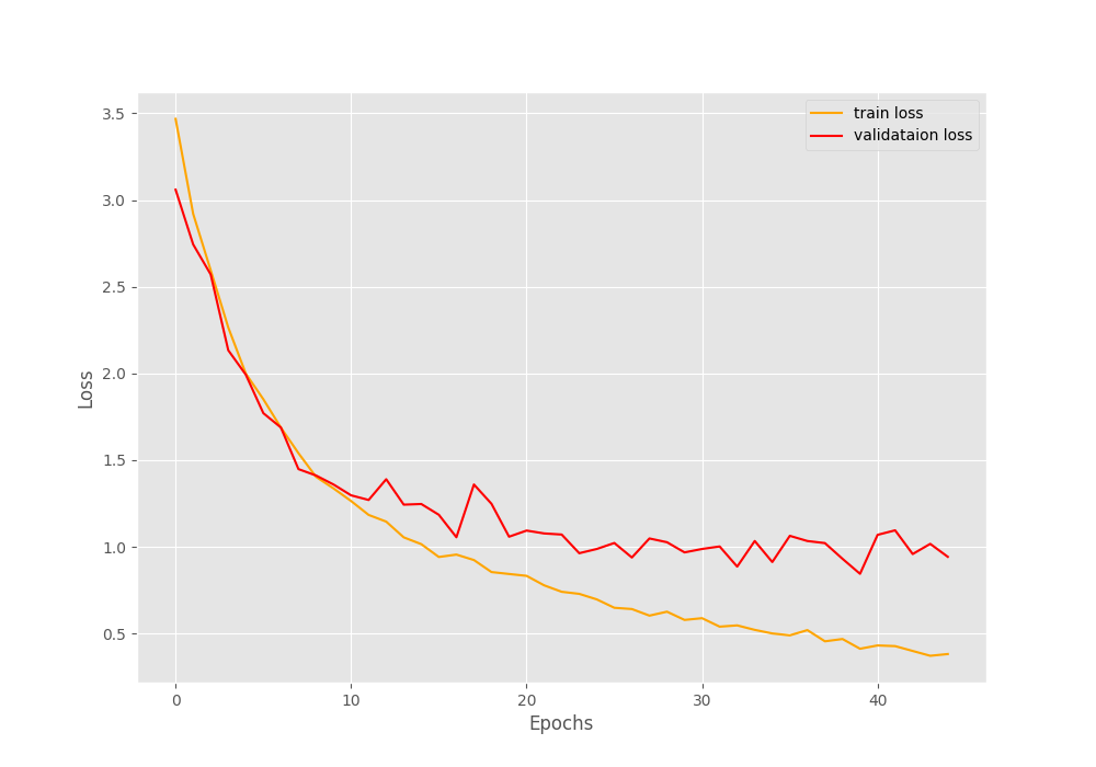
By the end of the training, the training accuracy is around 87.3%, and validation accuracy is 76.4%. The loss values stand at 0.381 and 0.942 for training and validation respectively.

From the loss graph, it looks like any more training would have resulted in the validation loss diverging from the training loss curve, at least under the current training settings. Hopefully, our model has learned well enough to classify most of the test images correctly.

The Inference Script

By now, we are done with the training part of the tutorial. Using the PyTorch ImageFolder for training CNN models made our work really easier. The only thing left is the inference. As we already have a trained model, let’s write a simple inference script to test our model on unseen images.

For testing, we will use images from the test subdirectory inside the butterflies_rev2 folder. The images are again inside their respective class directories, so, we can easily extract the ground truth information also.

The code that we will write here, will go into the inference.py script.

The first code block contains all the import statements and the construction of the argument parser.

import torch
import cv2
import torchvision.transforms as transforms
import argparse

from model import CNNModel

# construct the argument parser
parser = argparse.ArgumentParser()
parser.add_argument('-i', '--input', 
    default='input/butterflies_rev2/test/adonis/1.jpg',
    help='path to the input image')
args = vars(parser.parse_args())

The --input flag will take the path to the test image. We have provided a default path for a test image as well.

The next code block defines the computation device and all the class labels that we have.

# the computation device
device = ('cuda' if torch.cuda.is_available() else 'cpu')

# list containing all the class labels
labels = [
    'adonis', 'american snoot', 'an 88', 'banded peacock', 'beckers white', 
    'black hairstreak', 'cabbage white', 'chestnut', 'clodius parnassian', 
    'clouded sulphur', 'copper tail', 'crecent', 'crimson patch', 
    'eastern coma', 'gold banded', 'great eggfly', 'grey hairstreak', 
    'indra swallow', 'julia', 'large marble', 'malachite', 'mangrove skipper',
    'metalmark', 'monarch', 'morning cloak', 'orange oakleaf', 'orange tip', 
    'orchard swallow', 'painted lady', 'paper kite', 'peacock', 'pine white',
    'pipevine swallow', 'purple hairstreak', 'question mark', 'red admiral',
    'red spotted purple', 'scarce swallow', 'silver spot skipper', 
    'sixspot burnet', 'skipper', 'sootywing', 'southern dogface', 
    'straited queen', 'two barred flasher', 'ulyses', 'viceroy', 
    'wood satyr', 'yellow swallow tail', 'zebra long wing'
    ]

The labels list contains all the 50 class names that we have in the dataset.

Initialize the Model and Define the Preprocessing Tranforms

Now, we will initialize the model and load the trained weights.

# initialize the model and load the trained weights
model = CNNModel().to(device)
checkpoint = torch.load('outputs/model.pth', map_location=device)
model.load_state_dict(checkpoint['model_state_dict'])
model.eval()

Be sure to switch the model to eval() mode as we have done above for the proper behavior of dropout and batch normalization layers.

We will not need any augmentation transforms for inference, just the preprocessing transforms which the following code block defines.

# define preprocess transforms
transform = transforms.Compose([
    transforms.ToPILImage(),
    transforms.Resize(224),
    transforms.ToTensor(),
    transforms.Normalize(
        mean=[0.5, 0.5, 0.5],
        std=[0.5, 0.5, 0.5]
    )
])  

As we will be reading the image using cv2, therefore, we need to convert them to PIL image format first. Then resizing them to 224×224 dimensions, converting them to tensors, and applying the same normalization statistics as training.

Read the Image and Carry Out the Forward Pass

This is the final section, where we will read the image, preprocess it, and carry out the forward pass.

Let’s write the entire code first, then we will take a look at the explanation.

# read and preprocess the image
image = cv2.imread(args['input'])
# get the ground truth class
gt_class = args['input'].split('/')[-2]
orig_image = image.copy()
# convert to RGB format
image = cv2.cvtColor(image, cv2.COLOR_BGR2RGB)
image = transform(image)
# add batch dimension
image = torch.unsqueeze(image, 0)
with torch.no_grad():
    outputs = model(image.to(device))
output_label = torch.topk(outputs, 1)
pred_class = labels[int(output_label.indices)]
cv2.putText(orig_image, 
    f"GT: {gt_class}",
    (10, 25),
    cv2.FONT_HERSHEY_SIMPLEX, 
    0.6, (0, 255, 0), 2, cv2.LINE_AA
)
cv2.putText(orig_image, 
    f"Pred: {pred_class}",
    (10, 55),
    cv2.FONT_HERSHEY_SIMPLEX, 
    0.6, (0, 0, 255), 2, cv2.LINE_AA
)
print(f"GT: {gt_class}, pred: {pred_class}")
cv2.imshow('Result', orig_image)
cv2.waitKey(0)
cv2.imwrite(f"outputs/{gt_class}{args['input'].split('/')[-1].split('.')[0]}.png",
    orig_image)

• After reading the image, we are using the image path to extract the ground truth class name on line 50. We just split the file path by / and get the second last element which contains the class name, which happens to be the directory name as well.
• We create a copy of the original image for OpenCV annotations later on.
• Then we preprocess the image and feed it to the model on line 58.
• The outputs contains the predictions for the likelihood of all the 50 classes. At line 59, we get the top 1 prediction only and map that index to the labels list on line 60 to get the class name.
• After that we put the ground truth and prediction class name texts on the image using OpenCV annotations.
• Finally, we show the resulting image on screen and save it to disk as well.

This completes our inference code as well. Let’s execute the script and check the output for a few images.

Execute inference.py Script

Let’s execute the script with the default path, where the butterfly belongs to the adonis class.

python inference.py 

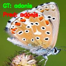
As we can see, our model is able to predict the class of the butterfly correctly, that is adonis.

Now, testing the model, where the butterfly belongs to the banded peacock class.

python inference.py -i "input/butterflies_rev2/test/banded peacock/1.jpg"

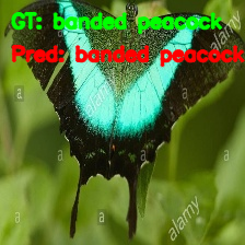
Our model is again able to predict the class correctly. Looks like the neural network model has learned the features of butterflies really well.

Now, one final test, for the great eggfly class.

python inference.py -i "input/butterflies_rev2/test/great eggfly/1.jpg"

This time also, the model is able to predict the class correctly.

A Few Takeaways

• Even with training from scratch and with such a simple model, our neural network model was able to predict three butterfly classes correctly. Although we were not able to carry out the predictions on all classes, the model seems to be performing well.
• The next step would be to use transfer learning and use a state-of-the-art pre-trained model for training and inference. That would surely give even better results.
• If you carry out transfer learning on your own, be sure to tell about your findings in the comment section. I am sure others will be interested to know.

Summary and Conclusion

In this tutorial, you learned how to use the ImageFolder class from PyTorch to easily prepare image classification datasets for training CNN models. Along with that, we also tackled a small yet interesting problem of classifying butterflies from 50 different species. I hope that you learned something new from this tutorial.

If you have any doubts, thoughts, or suggestions, then please leave them in the comment section. I will surely address them.

You can contact me using the Contact section. You can also find me on LinkedIn, and Twitter.