Cotton Disease Classification Using Vision Transformer and Visualizing Attention Maps

Vision Transformers have made their way into numerous useful Computer Vision applications. Although infamous for their huge data requirement, with the right strategy, we can fine-tune Vision Transformers even with a modest amount of data. We will try something similar in this article. We will fine-tune a Vision Transformer model for Cotton Disease Classification.

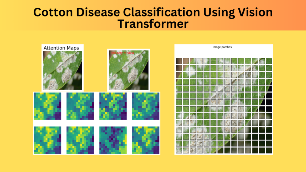
Along with fine-tuning, we will also visualize the attention maps on the validation dataset using the trained Vision Transformer model. This will pave the way towards explaining where the Transformer model looks when carrying out inference.

We will cover the following points in this article

• First, we are going to take a look at the dataset. This will give us clarity on what we are dealing with and how best to tackle it.
• Second, we will move to the coding part. Here, we will prepare the Vision Transformer model, the dataset, and other important scripts.
• Third, we will train the model and check its performance.
• Fourth, we will visualize the attention maps using the trained model on the validation set.
• Finally, we will discuss some models that were experimented with but did not work out well.

The Cotton Disease Dataset

We will use the Customized Cotton Disease Dataset for fine-tuning the Vision Transformer model.

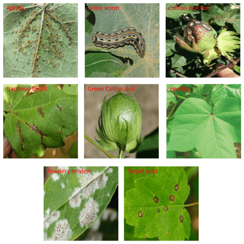
This dataset contains 8 classes including cotton diseases, healthy leaves, and healthy cotton balls.

• Aphids
• Army worm
• Bacterial blight
• Cotton Boll Rot
• Green Cotton Boll
• Healthy
• Powdery mildew
• Target spot

The dataset has been divided into a training and a validation set. There are 800 images for each class in the training set and between 40 to 60 images for each class in the validation set.

Here is a sample from each class of the training set.

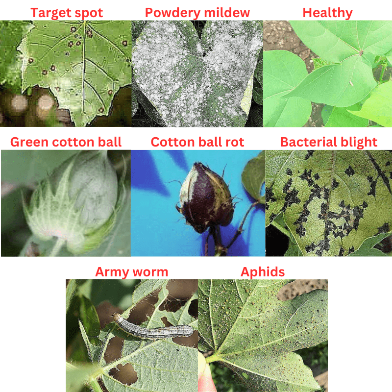
As we can see, the images are varied and even the same class contains diseased leaf images in different conditions.

Downloading and extracting the dataset will reveal the following directory structure.

├── Cotton-Disease-Training
│   └── trainning
│       └── Cotton leaves - Training
│           └── 800 Images
│               ├── Aphids
│               ├── Army worm
│               ├── Bacterial blight
│               ├── Cotton Boll Rot
│               ├── Green Cotton Boll
│               ├── Healthy
│               ├── Powdery mildew
│               └── Target spot
├── Cotton-Disease-Validation
│   └── validation
│       └── Cotton plant disease-Validation
│           └── Cotton plant disease-Validation
│               ├── Aphids edited
│               ├── Army worm edited
│               ├── Bacterial Blight edited
│               ├── Cotton Boll rot
│               ├── Green Cotton Boll
│               ├── Healthy leaf edited
│               ├── Powdery Mildew Edited
│               └── Target spot edited
└── Customized Cotton Dataset-Complete
    └── content
        ├── trainning
        │   └── Cotton leaves - Training
        │       └── 800 Images
        └── validation
            └── Cotton plant disease-Validation
                └── Cotton plant disease-Validation

The dataset has a deep nested structure. However, we are interested in the Cotton-Disease-Training and Cotton-Disease-Validation directories only.

Inside the respective data split directories, the class name subdirectories contain the images. You may have a detailed look on your own before moving to the next section.

Project Directory Structure

Let’s take a look at the entire project’s directory structure.

├── input
│   ├── Cotton-Disease-Training
│   ├── Cotton-Disease-Validation
│   └── Customized Cotton Dataset-Complete
├── outputs
│   ├── accuracy.png
│   ├── best_model.pth
│   ├── loss.png
│   └── model.pth
├── src
│   ├── datasets.py
│   ├── inference.py
│   ├── model.py
│   ├── train.py
│   └── utils.py
└── inference.ipynb

• As we saw in the previous section, the input directory contains the dataset.
• The outputs directory contains the trained models and the accuracy & loss graphs.
• The src directory contains all the source code.
• Finally, the inference.ipynb notebook is for running inference after training.

Setup for Training Vision Transformer for Cotton Disease Classification

We will use the vision_transformers library that I have been maintaining for a while now for training the model. It contains support for image classification and object detection training using Transformer models. For this, the base library is PyTorch. You can create a new environment and install the requirements.

First, install PyTorch

conda install pytorch torchvision torchaudio pytorch-cuda=11.8 -c pytorch -c nvidia

Then we need to clone the repository into the directory of choice, not necessarily the project directory.

git clone https://github.com/sovit-123/vision_transformers.git

Finally, enter the directory and install the library.

cd vision_transformers

pip install .

These are all the major deep learning library dependencies.

All the trained weights and source code will be available via the download section. You can directly run inference if you do not wish to run training by yourself.

Cotton Disease Classification using Vision Transformers

Let’s get started with the coding part.

For the most part, we will discuss the model preparation, the dataset preparation, and the training script.

Here are the steps we are going to follow for cotton disease classification.

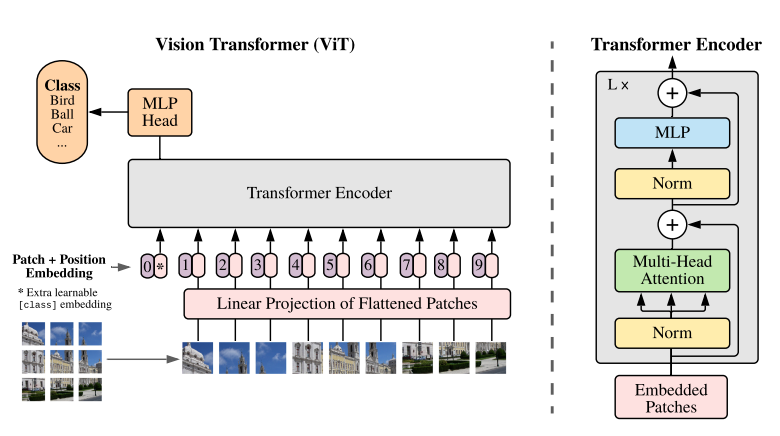
• We will start with the model preparation. We will use the ViT Base Patch 16 model which works on 224×224 images.
• Next, we will prepare the datasets and data loaders.
• Then, we will discuss the training script and start the training.
• After training, we will run inference on validation images and visualize the attention maps of the same.

Download Code

The Vision Transformer Model

Preparing the Vision Transformer model with the installed library is straightforward. It’s just a few lines of code. The following code goes into the model.py file.

from vision_transformers.models import vit

def build_model(num_classes=10):
    model = vit.vit_b_p16_224(
        image_size=224,
        num_classes=num_classes,
        pretrained=True
    )
    return model

if __name__ == '__main__':
    model = build_model()
    print(model)
    # Total parameters and trainable parameters.
    total_params = sum(p.numel() for p in model.parameters())
    print(f"{total_params:,} total parameters.")
    total_trainable_params = sum(
        p.numel() for p in model.parameters() if p.requires_grad)
    print(f"{total_trainable_params:,} training parameters.")

We have a build_model function that accepts the number of classes as the parameter. We initialize the model using the vit module of the vision_transformers library. It accepts the image size, the number of classes, and whether to load the pretrained weights or not as parameters.

This is all we need to prepare the Vision Transformer model.

If you wish to know the details of Vision Transformer, then you should surely give the Vision Transformer from scratch article a read.

Preparing the Datasets and Data Loaders

As we have the training and validation data in separate folders, we can use the PyTorch ImageFolder class to prepare the datasets.

The dataset preparation code goes into the datasets.py file.

Let’s start with the imports and define a few constants.

import os

from torchvision import datasets, transforms
from torch.utils.data import DataLoader

# Required constants.
TRAIN_DIR = os.path.join('../input/Cotton-Disease-Training/trainning/Cotton leaves - Training/800 Images')
VALID_DIR = os.path.join('../input/Cotton-Disease-Validation/validation/Cotton plant disease-Validation/Cotton plant disease-Validation')
IMAGE_SIZE = 224 # Image size of resize when applying transforms.
NUM_WORKERS = 4 # Number of parallel processes for data preparation.

We define the paths to the training and validation data along with the image size and number of workers for the data loaders.

Next, let’s define the training and validation transforms.

# Training transforms
def get_train_transform(image_size):
    train_transform = transforms.Compose([
        transforms.Resize((image_size, image_size)),
        transforms.RandomHorizontalFlip(p=0.5),
        transforms.RandomRotation(35),
        transforms.RandomAdjustSharpness(sharpness_factor=2, p=0.5),
        transforms.ToTensor(),
        transforms.Normalize(
            mean=[0.485, 0.456, 0.406],
            std=[0.229, 0.224, 0.225]
            )
    ])
    return train_transform

# Validation transforms
def get_valid_transform(image_size):
    valid_transform = transforms.Compose([
        transforms.Resize((image_size, image_size)),
        transforms.ToTensor(),
        transforms.Normalize(
            mean=[0.485, 0.456, 0.406],
            std=[0.229, 0.224, 0.225]
            )
    ])
    return valid_transform

For training, along with ImageNet normalization, we apply the following image augmentation.

• Random horizontal flipping
• Random rotation
• Adjusting sharpness randomly

For validation, we just resize the images and apply ImageNet normalization.

The final two functions are for preparing the datasets and the data loaders.

def get_datasets():
    """
    Function to prepare the Datasets.
    Returns the training and validation datasets along 
    with the class names.
    """
    dataset_train = datasets.ImageFolder(
        TRAIN_DIR, 
        transform=(get_train_transform(IMAGE_SIZE))
    )
    dataset_valid = datasets.ImageFolder(
        VALID_DIR, 
        transform=(get_valid_transform(IMAGE_SIZE))
    )
    return dataset_train, dataset_valid, dataset_train.classes

def get_data_loaders(dataset_train, dataset_valid, batch_size):
    """
    Prepares the training and validation data loaders.
    :param dataset_train: The training dataset.
    :param dataset_valid: The validation dataset.
    Returns the training and validation data loaders.
    """
    train_loader = DataLoader(
        dataset_train, batch_size=batch_size, 
        shuffle=True, num_workers=NUM_WORKERS
    )
    valid_loader = DataLoader(
        dataset_valid, batch_size=batch_size, 
        shuffle=False, num_workers=NUM_WORKERS
    )
    return train_loader, valid_loader 

With this, we are done with the dataset preparation for cotton image classification.

The Training Script

Let’s get down to one of the most important files, the train.py file. This is the driver script that we will execute to start the training.

The following lines cover the import statements, setting of the seed, and defining the argument parser.

import torch
import argparse
import torch.nn as nn
import torch.optim as optim
import os

from tqdm.auto import tqdm
from model import build_model
from datasets import get_datasets, get_data_loaders
from utils import save_model, save_plots, SaveBestModel
from torch.optim.lr_scheduler import MultiStepLR

seed = 42
torch.manual_seed(seed)
torch.cuda.manual_seed(seed)
torch.backends.cudnn.deterministic = True
torch.backends.cudnn.benchmark = True

# Construct the argument parser.
parser = argparse.ArgumentParser()
parser.add_argument(
    '-e', '--epochs', 
    type=int, 
    default=10,
    help='Number of epochs to train our network for'
)
parser.add_argument(
    '-lr', '--learning-rate', 
    type=float,
    dest='learning_rate', 
    default=0.001,
    help='Learning rate for training the model'
)
parser.add_argument(
    '-b', '--batch-size',
    dest='batch_size',
    default=32,
    type=int
)
parser.add_argument(
    '--save-name',
    dest='save_name',
    default='model',
    help='file name of the final model to save'
)
args = vars(parser.parse_args())

For the argument parser, we have:

• --epochs: The number of epochs we want to train the model for.
• --learning-rate: Base learning rate for the optimizer.
• --batch-size: Batch size for the data loaders.
• --save-name: The name of the saved model file. By default, it is model.pth.

Next, we have the generic training and validation functions for PyTorch image classification.

# Training function.
def train(model, trainloader, optimizer, criterion):
    model.train()
    print('Training')
    train_running_loss = 0.0
    train_running_correct = 0
    counter = 0
    for i, data in tqdm(enumerate(trainloader), total=len(trainloader)):
        counter += 1
        image, labels = data
        image = image.to(device)
        labels = labels.to(device)
        optimizer.zero_grad()
        # Forward pass.
        outputs = model(image)
        # Calculate the loss.
        loss = criterion(outputs, labels)
        train_running_loss += loss.item()
        # Calculate the accuracy.
        _, preds = torch.max(outputs.data, 1)
        train_running_correct += (preds == labels).sum().item()
        # Backpropagation.
        loss.backward()
        # Update the weights.
        optimizer.step()
    
    # Loss and accuracy for the complete epoch.
    epoch_loss = train_running_loss / counter
    epoch_acc = 100. * (train_running_correct / len(trainloader.dataset))
    return epoch_loss, epoch_acc

# Validation function.
def validate(model, testloader, criterion, class_names):
    model.eval()
    print('Validation')
    valid_running_loss = 0.0
    valid_running_correct = 0
    counter = 0

    with torch.no_grad():
        for i, data in tqdm(enumerate(testloader), total=len(testloader)):
            counter += 1
            
            image, labels = data
            image = image.to(device)
            labels = labels.to(device)
            # Forward pass.
            outputs = model(image)
            # Calculate the loss.
            loss = criterion(outputs, labels)
            valid_running_loss += loss.item()
            # Calculate the accuracy.
            _, preds = torch.max(outputs.data, 1)
            valid_running_correct += (preds == labels).sum().item()
        
    # Loss and accuracy for the complete epoch.
    epoch_loss = valid_running_loss / counter
    epoch_acc = 100. * (valid_running_correct / len(testloader.dataset))
    return epoch_loss, epoch_acc

Finally, we have the main block.

if __name__ == '__main__':
    # Create a directory with the model name for outputs.
    out_dir = os.path.join('..', 'outputs')
    os.makedirs(out_dir, exist_ok=True)
    # Load the training and validation datasets.
    dataset_train, dataset_valid, dataset_classes = get_datasets()
    print(f"[INFO]: Number of training images: {len(dataset_train)}")
    print(f"[INFO]: Number of validation images: {len(dataset_valid)}")
    print(f"[INFO]: Classes: {dataset_classes}")
    # Load the training and validation data loaders.
    train_loader, valid_loader = get_data_loaders(
        dataset_train, dataset_valid, batch_size=args['batch_size']
    )

    # Learning_parameters. 
    lr = args['learning_rate']
    epochs = args['epochs']
    device = ('cuda' if torch.cuda.is_available() else 'cpu')
    print(f"Computation device: {device}")
    print(f"Learning rate: {lr}")
    print(f"Epochs to train for: {epochs}\n")

    # Load the model.
    model = build_model(
        num_classes=len(dataset_classes)
    ).to(device)
    print(model)
    
    # Total parameters and trainable parameters.
    total_params = sum(p.numel() for p in model.parameters())
    print(f"{total_params:,} total parameters.")
    total_trainable_params = sum(
        p.numel() for p in model.parameters() if p.requires_grad)
    print(f"{total_trainable_params:,} training parameters.")

    # Optimizer.
    optimizer = optim.SGD(
        model.parameters(), lr=lr, momentum=0.9, nesterov=True
    )
    # Loss function.
    criterion = nn.CrossEntropyLoss()

    # Initialize `SaveBestModel` class.
    save_best_model = SaveBestModel()

    # Scheduler.
    scheduler = MultiStepLR(
        optimizer, milestones=[10], gamma=0.1, verbose=True
    )

    # Lists to keep track of losses and accuracies.
    train_loss, valid_loss = [], []
    train_acc, valid_acc = [], []
    # Start the training.
    for epoch in range(epochs):
        print(f"[INFO]: Epoch {epoch+1} of {epochs}")
        train_epoch_loss, train_epoch_acc = train(model, train_loader, 
                                                optimizer, criterion)
        valid_epoch_loss, valid_epoch_acc = validate(model, valid_loader,  
                                                    criterion, dataset_classes)
        train_loss.append(train_epoch_loss)
        valid_loss.append(valid_epoch_loss)
        train_acc.append(train_epoch_acc)
        valid_acc.append(valid_epoch_acc)
        print(f"Training loss: {train_epoch_loss:.3f}, training acc: {train_epoch_acc:.3f}")
        print(f"Validation loss: {valid_epoch_loss:.3f}, validation acc: {valid_epoch_acc:.3f}")
        save_best_model(
            valid_epoch_loss, epoch, model, out_dir, args['save_name']
        )
        print('-'*50)
        scheduler.step()

    # Save the trained model weights.
    save_model(epochs, model, optimizer, criterion, out_dir, args['save_name'])
    # Save the loss and accuracy plots.
    save_plots(train_acc, valid_acc, train_loss, valid_loss, out_dir)
    print('TRAINING COMPLETE')

First, we prepare the datasets and data loaders.

Second, we initialize the model, the optimizer, the loss function, and the Multi-Step Learning Rate Scheduler.

Third, we start the training loop and save the best model whenever the current epoch’s loss is less than the previous least loss.

This finishes the training script code as well.

We also have a utils.py file which contains helper functions to save models and accuracy & loss graphs. You may have a look at it before moving to the training section.

Training the Vision Transformer Model for Cotton Disease Classification

We can execute the following command within the src directory to start the training.

python train.py -lr 0.0005 --epochs 15 --batch 32

We start with a base learning rate of 0.0005, batch size of 32, and train for 15 epochs.

Here are the logs.

[INFO]: Epoch 1 of 15
Training
100%|████████████████████████████████████████████████████████████████████████████████████████████████████████████████████████████████████████████████████████████████████████████| 208/208 [00:51<00:00,  4.08it/s]
Validation
100%|██████████████████████████████████████████████████████████████████████████████████████████████████████████████████████████████████████████████████████████████████████████████| 12/12 [00:01<00:00,  8.36it/s]
Training loss: 0.584, training acc: 85.576
Validation loss: 0.179, validation acc: 94.958

Best validation loss: 0.179245263338089

Saving best model for epoch: 1

--------------------------------------------------
Adjusting learning rate of group 0 to 5.0000e-04.
[INFO]: Epoch 2 of 15
Training
100%|████████████████████████████████████████████████████████████████████████████████████████████████████████████████████████████████████████████████████████████████████████████| 208/208 [00:50<00:00,  4.09it/s]
Validation
100%|██████████████████████████████████████████████████████████████████████████████████████████████████████████████████████████████████████████████████████████████████████████████| 12/12 [00:01<00:00,  8.42it/s]
Training loss: 0.087, training acc: 98.295
Validation loss: 0.107, validation acc: 96.639

Best validation loss: 0.10733319881061713

Saving best model for epoch: 2

--------------------------------------------------
.
.
.
Adjusting learning rate of group 0 to 5.0000e-05.
[INFO]: Epoch 15 of 15
Training
100%|████████████████████████████████████████████████████████████████████████████████████████████████████████████████████████████████████████████████████████████████████████████| 208/208 [00:50<00:00,  4.12it/s]
Validation
100%|██████████████████████████████████████████████████████████████████████████████████████████████████████████████████████████████████████████████████████████████████████████████| 12/12 [00:01<00:00,  8.41it/s]
Training loss: 0.006, training acc: 99.894
Validation loss: 0.098, validation acc: 97.199
--------------------------------------------------
Adjusting learning rate of group 0 to 5.0000e-05.
TRAINING COMPLETE

The validation accuracy almost plateaued out after 5 epochs. We get the best model after epoch 5 with a validation accuracy of 97.75% and a validation loss of 0.089.

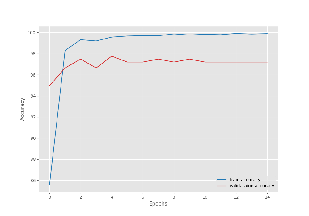
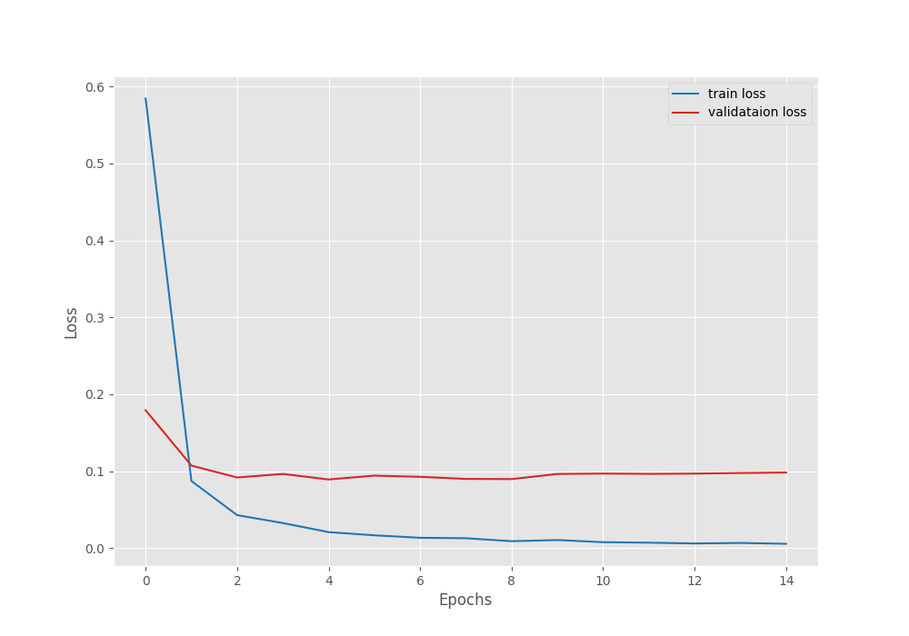
From the graphs, it is clear that the validation plots started deteriorating after 5 epochs. Most probably, adding more augmentations and a more aggressive learning rate scheduler will work better.

Inference and Visualizing Attention Maps

You can run the inference.py script as well for inference on the images in input/inference_data directory. However, here, we will follow the inference.ipynb notebook for inference and visualizing the attention maps.

Starting with the required imports and setting up the computation device.

import torch
import torchvision.transforms as transforms
import numpy as np
import matplotlib.pyplot as plt
import glob

from PIL import Image
from vision_transformers.models import vit

device = torch.device('cuda:0' if torch.cuda.is_available() else 'cpu')

Next, let’s define the class names, initialize the model, and load the trained weights.

class_names = [
    'Aphids', 
    'Army worm', 
    'Bacterial blight', 
    'Cotton Boll Rot', 
    'Green Cotton Boll', 
    'Healthy', 
    'Powdery mildew', 
    'Target spot'
]

model = vit.vit_b_p16_224(num_classes=len(class_names), pretrained=False).eval()
ckpt = torch.load('outputs/best_model.pth')
model.load_state_dict(ckpt['model_state_dict'])

Now, defining the transforms and carrying out the inference.

transform = transforms.Compose([
    transforms.ToTensor(),
    transforms.Normalize(
        mean = [0.485, 0.456, 0.406],
        std = [0.229, 0.224, 0.225]
    )
])

def infer(image_path):
    image = Image.open(image_path)
    image = image.resize((224, 224))
    plt.figure(figsize=(6, 3))
    plt.imshow(image)
    plt.axis('off')
    input_tensor = transform(image).unsqueeze(0)
    with torch.no_grad():
        output = model(input_tensor)
    
    probabilities = torch.nn.functional.softmax(output[0], dim=0)
    probabilities = probabilities.numpy()
    category = class_names[np.argmax(probabilities)]
    plt.text(x=10, y=20, s=category, fontsize='large', color='red')
    plt.show()

image_paths = glob.glob('input/inference_data/*')
for i, image_path in enumerate(image_paths):
    if i == 10:
        break
    infer(image_path)

We use one image from each class of the validation dataset for inference. Here are the results.

Surprisingly, the trained Vision Transformer model can classify all the images correctly.

Visualizing Attention Maps

Visualizing the attention maps for the cotton disease classification will reveal which area the model attends to when classifying an image. We have covered an in-depth explanation of visualizing attention maps in the article where we fine-tuned the Vision Transformer.

Here, we will cover the code with an overview explanation.

First, let’s load the model onto the CPU and read an image.

model = model.cpu()

image = Image.open('input/inference_data/powdery_mildew.jpg')
image = image.resize((224, 224))
input_tensor = transform(image).unsqueeze(0)

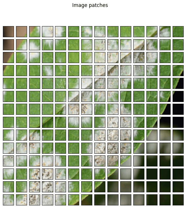
The first step is converting the images to patches.

# Patch embedding.
patches = model.patches.patch(input_tensor)
print(f"Input tensor shape: {input_tensor.shape}")
print(f"Patch embedding shape: {patches.shape}")

fig = plt.figure(figsize=(8, 8))
fig.suptitle("Image patches", fontsize=12)
img = np.asarray(image)
for i in range(0, 196):
    x = i % 14
    y = i // 14
    patch = img[y*16:(y+1)*16, x*16:(x+1)*16]
    ax = fig.add_subplot(14, 14, i+1)
    ax.axes.get_xaxis().set_visible(False)
    ax.axes.get_yaxis().set_visible(False)
    ax.imshow(patch)

The following image shows what happens when we convert a 224×224 image to 16×16 patches.

Next, we compute the positional embeddings and the attention matrix.

pos_embed = model.pos_embedding
print(pos_embed.shape)

patch_input = patches.view(1, 768, 196).permute(0, 2, 1)
print(patch_input.shape)

transformer_input = torch.cat((model.cls_token, patch_input), dim=1) + pos_embed
print("Transformer input: ", transformer_input.shape)

transformer_input_qkv = model.transformer.layers[0][0].fn.qkv(transformer_input)[0]
print(transformer_input_qkv.shape)

qkv = transformer_input_qkv.reshape(197, 3, 12, 64)
print("Reshaped qkv : ", qkv.shape)
q = qkv[:, 0].permute(1, 0, 2)
k = qkv[:, 1].permute(1, 0, 2)
kT = k.permute(0, 2, 1)
print("K transposed: ", kT.shape)

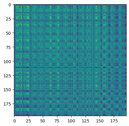
# Attention Matrix
attention_matrix = q @ kT
print("Attention matrix: ", attention_matrix.shape)
plt.imshow(attention_matrix[3].detach().cpu().numpy())

The final step is visualizing the attention maps.

# Visualize attention matrix
fig = plt.figure(figsize=(6, 3))
fig.suptitle("Attention Maps", fontsize=20)
# fig.add_axes()
img = np.asarray(img)
ax1 = fig.add_subplot(1, 1, 1)
ax1.imshow(img)
ax1.axis('off')
fig = plt.figure(figsize=(16, 8))
for i in range(8):
    attn_heatmap = attention_matrix[i, 64, 1:].reshape((14, 14)).detach().cpu().numpy()
    ax2 = fig.add_subplot(2, 4, i+1)
    ax2.imshow(attn_heatmap)
    ax2.axis('off')

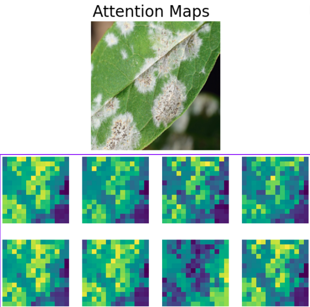
The above image makes it very clear how the model focuses on the white diseased part of the leaf. It becomes easier for us to interpret the output of the model and to infer why it made a certain decision.

Vision Transformer Models that Did Not Work

Among other ViT models, models that create 32×32 resolution patches and ViT Tiny models did not work very well. Mostly, ViT models need smaller patches, e.g. 16×16 to properly learn the features of the diseased leaves. Furthermore, the ViT Tiny models may not have the capacity to learn complex features when the dataset is not large.

Summary and Conclusion

In this article, we went through the classification of cotton disease using the Vision Transformer model. Along with the fine-tuning of the Vision Transformer, we also ran inference and visualized the attention maps. This gave us a much better idea of how the model makes the decisions. I hope that this article was worth your time.

If you have any doubts, thoughts, or suggestions, please leave them in the comment section. I will surely address them.

You can contact me using the Contact section. You can also find me on LinkedIn, and Twitter.