Fine Tuning Vision Transformer and Visualizing Attention Maps

Vision transformers have become the go-to model for a lot of computer vision based deep learning tasks. Be it image classification, object detection, or image segmentation. They are outperforming CNN based models in most of the tasks. With such wide adoption, fine tuning vision transformers is easier now than ever. Although primarily it is the same as fine-tuning any other image classification model, getting hands-on never hurts. In this article, we will be fine tuning a Vision Transformer model and also visualize the attention maps during inference.

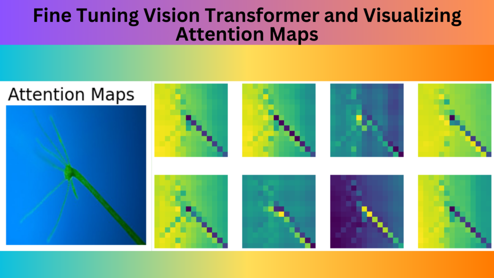
In Convolutional Neural Networks, we visualize activation maps to know where the model focuses. Similarly, we can visualize the attention maps in transformer based models. The above is such an example of attention map visualization in the Vision Transformer (ViT) model.

Following are the topics that we will cover in this article:

• We will start with the exploration of the dataset. We will use a fairly small microorganism dataset from Kaggle.
• Then we will move on to the setup of the vision_transformers library that we will use to fine tune the ViT model.
• Next, we will discuss some implementation and dataset related details.
• Then we will move on to training the model.
• After training, we will carry out inference and visualize the attention maps for the inference images.

Note: We will not get into the theoretical explanation of the attention maps in Vision Transformers in this article. We will take a complete coding approach here.

The Microorganism Classification Dataset

We will use the Micro-Organism Image Classification dataset in this article for fine tuning the Vision Transformer model.

The dataset contains images of 8 different types of microorganisms. So, there are 8 classes, and images related to each class reside inside their respective folders.

Here are the 8 classes.

• Amoeba
• Euglena
• Hydra
• Paramecium
• Rod bacteria
• Spherical bacteria
• Spiral bacteria
• Yeast

The dataset is imbalanced and each class contains somewhere between 70 to 200 images. Here are a few samples from the dataset.

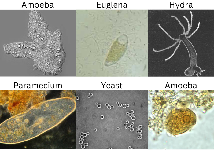
As we can see, the images are quite varied even within the same class. It may prove slightly difficult for the model to achieve very high accuracy with such a small set of samples.

After downloading and extracting the dataset, you should see the following structure.

Micro_Organism/
├── Amoeba [72 entries exceeds filelimit, not opening dir]
├── Euglena [168 entries exceeds filelimit, not opening dir]
├── Hydra [76 entries exceeds filelimit, not opening dir]
├── Paramecium [152 entries exceeds filelimit, not opening dir]
├── Rod_bacteria [85 entries exceeds filelimit, not opening dir]
├── Spherical_bacteria [86 entries exceeds filelimit, not opening dir]
├── Spiral_bacteria [75 entries exceeds filelimit, not opening dir]
└── Yeast [75 entries exceeds filelimit, not opening dir] 

If you plan on running the training experiments, please go ahead and download the dataset from here.

Download Code

Setting up the vision_transformers Library

We will use the vision_transformers library to fine tune the ViT model. I have been maintaining this library for some time now. It has functionalities to train several transformer based image classification and DETR based object detection models.

In this article, we will only focus on the classification modules.

Please go ahead and clone the repository in the directory of your choice. Then enter the vision_transformers directory.

git clone https://github.com/sovit-123/vision_transformers.git

cd vision_transformers

First, let’s install the latest version of PyTorch with CUDA support using conda.

conda install pytorch torchvision torchaudio pytorch-cuda=11.7 -c pytorch -c nvidia

Then install the library.

pip install .

Next, install all other requirements.

pip install -r requirements.txt

That’s all we need to set up the vision_transformers library.

The Project Directory Structure

Here is the final project directory structure.

├── input
│   ├── inference_data
│   │   ├── amoeba.jpg
│   │   ├── euglena.jpg
│   │   ├── hydra.jpg
│   │   └── yeast.jpg
│   ├── Micro_Organism
│   │   ├── Amoeba [72 entries exceeds filelimit, not opening dir]
│   │   ├── Euglena [168 entries exceeds filelimit, not opening dir]
│   │   ├── Hydra [76 entries exceeds filelimit, not opening dir]
│   │   ├── Paramecium [152 entries exceeds filelimit, not opening dir]
│   │   ├── Rod_bacteria [85 entries exceeds filelimit, not opening dir]
│   │   ├── Spherical_bacteria [86 entries exceeds filelimit, not opening dir]
│   │   ├── Spiral_bacteria [75 entries exceeds filelimit, not opening dir]
│   │   └── Yeast [75 entries exceeds filelimit, not opening dir]
│   └── microorganism-image-classification.zip
├── vision_transformers
│   ├── data
│   │   ├── aquarium.yaml
│   │   ├── test_image_config.yaml
│   │   └── test_video_config.yaml
│   ├── examples
│   │   ...
│   ├── example_test_data
│   │   ...
│   ├── readme_images
│   │   ├── detr_infer.gif
│   │   └── detr.png
│   ├── runs
│   ├── tools
│   │   ├── utils
│   │   ├── export.py
│   │   ├── inference_image_detect.py
│   │   ├── inference_video_detect.py
│   │   ├── __init__.py
│   │   ├── onnx_infer_image_detect.py
│   │   ├── onnx_infer_video_detect.py
│   │   ├── train_classifier.py
│   │   └── train_detector.py
│   ├── vision_transformers
│   │   ├── detection
│   │   ...
│   │   └── __init__.py
│   ├── LICENSE
│   ├── README.md
│   ├── requirements.txt
│   └── setup.py
└── attention_microorganisms.ipynb

• Inside the project directory, first, we have the input directory. This contains the training dataset that we saw earlier. Along with that, it also contains an inference directory with a few images that we will run inference on.
• The cloned vision_transformers directory contains a lot of subdirectories. However, we are most interested in the dataset and training scripts present inside the tools directory. We will get into more details while using the necessary scripts.
• Directly inside the project directory, we have attention_microorganisms.ipynb notebook. We will use this for running inference and visualizing the attention maps of the vision transformer model.

The inference data, trained weights, and the notebook for visualizing attention maps are available to download via the code download section. If you just wish to run inference, you can download the code, extract it and copy the runs folder into the cloned vision_transformers directory.

Implementation Details of Fine Tuning Vision Transformer Model

In case you plan on training the model using the commands in the following sections, please ensure that you have downloaded the dataset and set up the directory as per the above structure.

The Vision Transformer Model Details

We will be fine tuning the ViT Base Model which coverts the input images to 16×16 patches. Commonly, this model is known as ViT_B_P16_224. The 224 at the end indicates that the images will be resized into 224×224 resolution internally by the dataloader.

In the vision_transformers library, it has the model flag name of vit_b_p16_224. It is almost the same as the model that we can find in the original Vision Transformer paper.

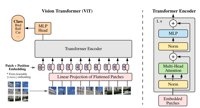
In the library, the model has been implemented from the ground up to make it more modular. This allows easy access to the layers. During run time, when fine tuning, the PyTorch ViT pretrained weights are loaded.

You can find more implementation details inside the vision_transformers/models/vit.py file.

The Data Loader Details

At the time of writing this, the data loader is quite simple. This will surely change in the future. It does not apply any image augmentations by default. The image classification data loader code is present inside tools/utils/dataloader.py.

It expects that the dataset should contain all the images inside their respective class folders. They can either have separate train and validation split directories or can be a single directory. But the images being present in the class folders is a hard requirement to make use of the ImageFolder class from PyTorch.

Fine Tuning the Vision Transformer Model

Fine tuning the Vision Transformer model using this library is quite easy. We just need to execute a single script with the necessary command line arguments.

For this, we will execute the train_classifier.py file inside the tools directory. Let’s start. To start the training, we need to execute the following command inside the cloned vision_transformers directory.

python tools/train_classifier.py --data-dir ../input/Micro_Organism/ 0.15 -lr 0.0001 --epochs 70 --batch 32 --name micro

We use the following command line arguments:

• --data-dir: This accepts multiple arguments. As you may remember, we do not have training and validation splits in our dataset. So, we use this flag first to point to the dataset directory path. The second argument is the validation split which is 0.15 in this case.
• -lr: This is the learning rate that we want to use. We use a very low learning rate of 0.0001.
• --epochs: The number of epochs that we want to train for. Here, we are training for 70 epochs.
• --batch: This accepts the batch size for the data loader. Higher batch sizes generally give good results in most transformer based models. We use a batch size of 32 in our case.
• --name: This is the resulting directory name that will be generated inside runs/training. All the graphs, logs, and trained weights will be saved here.

The training should not take long considering that we do not use a very big dataset.

Training Results

The following block shows the training logs from the final few epochs.

[INFO]: Epoch 67 of 70
Training
100%|██████████████████████████████████████████████████████████████████████████████████████████████████████████████████████████████████████████████████████████████████████████████| 21/21 [00:05<00:00,  3.67it/s]
Validation
100%|████████████████████████████████████████████████████████████████████████████████████████████████████████████████████████████████████████████████████████████████████████████████| 4/4 [00:00<00:00,  5.87it/s]

LOWEST VALIDATION LOSS: 0.9860654026269913

SAVING BEST MODEL FOR EPOCH: 67

SAVING PLOTS COMPLETE...
Training loss: 0.118, training acc: 98.212
Validation loss: 0.986, validation acc: 67.797
--------------------------------------------------
[INFO]: Epoch 68 of 70
Training
100%|██████████████████████████████████████████████████████████████████████████████████████████████████████████████████████████████████████████████████████████████████████████████| 21/21 [00:06<00:00,  3.42it/s]
Validation
100%|████████████████████████████████████████████████████████████████████████████████████████████████████████████████████████████████████████████████████████████████████████████████| 4/4 [00:00<00:00,  5.46it/s]
SAVING PLOTS COMPLETE...
Training loss: 0.114, training acc: 98.659
Validation loss: 0.988, validation acc: 67.797
--------------------------------------------------
[INFO]: Epoch 69 of 70
Training
100%|██████████████████████████████████████████████████████████████████████████████████████████████████████████████████████████████████████████████████████████████████████████████| 21/21 [00:06<00:00,  3.50it/s]
Validation
100%|████████████████████████████████████████████████████████████████████████████████████████████████████████████████████████████████████████████████████████████████████████████████| 4/4 [00:00<00:00,  5.79it/s]
SAVING PLOTS COMPLETE...
Training loss: 0.113, training acc: 97.914
Validation loss: 0.988, validation acc: 67.797
--------------------------------------------------
[INFO]: Epoch 70 of 70
Training
100%|██████████████████████████████████████████████████████████████████████████████████████████████████████████████████████████████████████████████████████████████████████████████| 21/21 [00:05<00:00,  3.88it/s]
Validation
100%|████████████████████████████████████████████████████████████████████████████████████████████████████████████████████████████████████████████████████████████████████████████████| 4/4 [00:00<00:00,  5.67it/s]
SAVING PLOTS COMPLETE...
Training loss: 0.109, training acc: 98.361
Validation loss: 0.990, validation acc: 66.949
--------------------------------------------------
TRAINING COMPLETE

We get the best model according to the least loss on epoch 67. The validation loss is 0.98 and the validation accuracy is 67.97%.

This is not too high but again, we did not use any augmentations, so, training for longer may lead to overfitting.

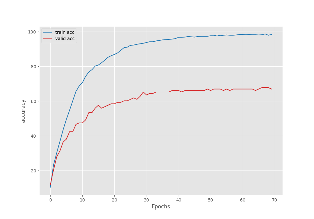
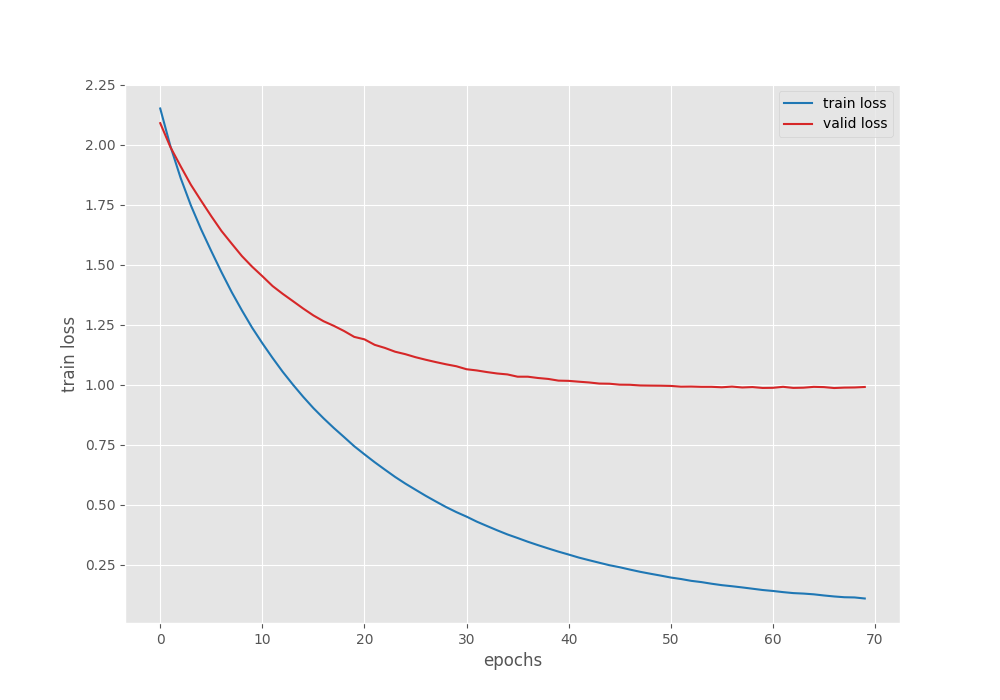
We can see that the validation accuracy and loss plots have almost plateaued out. The only ways we can have better results are by using augmentations or adding more data.

However, for now, we have a fine tuned Vision Transformer model. Let’s move ahead with the inference and visualization of the attention maps.

Inference using Trained Vision Transformer Model and Visualizing Attention Maps

Let’s run inference and visualize attention maps using the trained Vision Transformer model now.

We will follow the attention_microorganisms.ipynb Jupyter Notebook for this.

Inference on Images

Let’s first import all the required libraries.

import torch
import torchvision.transforms as transforms
import numpy as np
import matplotlib.pyplot as plt
import numpy as np
import glob

from PIL import Image
from vision_transformers.models import vit

Next, define all the class names.

class_names = [
    'Amoeba', 
    'Euglena', 
    'Hydra', 
    'Paramecium', 
    'Rod_bacteria', 
    'Spherical_bacteria', 
    'Spiral_bacteria', 
    'Yeast'
]

Then load the fine tuned Vision Transformer model.

model = vit.vit_b_p16_224(num_classes=len(class_names), pretrained=True).eval()
ckpt = torch.load('vision_transformers/runs/training/micro/best_model.pth')
model.load_state_dict(ckpt['model_state_dict'])

The next code cell defines the transforms and an infer() function to carry out inference.

transform = transforms.Compose([
    transforms.ToTensor(),
    transforms.Normalize(
        mean = [0.485, 0.456, 0.406],
        std = [0.229, 0.224, 0.225]
    )
])

def infer(image_path):
    image = Image.open(image_path)
    image = image.resize((224, 224))
    plt.figure(figsize=(6, 3))
    plt.imshow(image)
    plt.title(image_path)
    plt.axis('off')
    input_tensor = transform(image).unsqueeze(0)
    with torch.no_grad():
        output = model(input_tensor)
    
    probabilities = torch.nn.functional.softmax(output[0], dim=0)
    probabilities = probabilities.numpy()
    category = class_names[np.argmax(probabilities)]
    plt.text(x=10, y=20, s=category, fontsize='large')
    plt.show()

image_paths = glob.glob('input/inference_data/*')
for image_path in image_paths:
    infer(image_path)

Here are the results from the cell outputs.

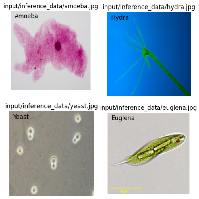
The path on the top of each image represents ground truth and the text inside the image represents the predictions. As we can see, the fine tuned Vision Transformer model is able to predict each class correctly.

Visualizing the Attention Maps

After fine tuning the Vision Transformer model, now, we can visualize the attention maps on one of the images used for inference.

Continuing with the notebook, let’s open the Hydra image and resize it to 224×224 resolution.

image = Image.open('input/inference_data/hydra.jpg')
image = image.resize((224, 224))
input_tensor = transform(image).unsqueeze(0)

Next, let’s compute the patches and visualize them.

# Patch embedding.
patches = model.patches.patch(input_tensor)
print(f"Input tensor shape: {input_tensor.shape}")
print(f"Patch embedding shape: {patches.shape}")

fig = plt.figure(figsize=(8, 8))
fig.suptitle("Image patches", fontsize=12)
img = np.asarray(image)
for i in range(0, 196):
    x = i % 14
    y = i // 14
    patch = img[y*16:(y+1)*16, x*16:(x+1)*16]
    ax = fig.add_subplot(14, 14, i+1)
    ax.axes.get_xaxis().set_visible(False)
    ax.axes.get_yaxis().set_visible(False)
    ax.imshow(patch)

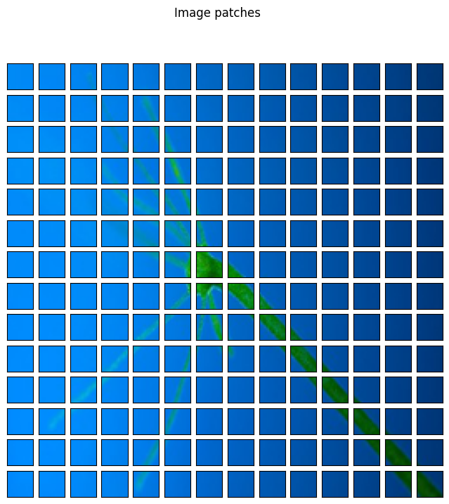
So, the model first converts the 224×224 image into 14×14 patches by passing it through a 2D Convolutional layer.

Then, we need to compute the positional embedding of the patches and reshape the patches as well.

pos_embed = model.pos_embedding
print(pos_embed.shape)
patch_input = patches.view(1, 768, 196).permute(0, 2, 1)
print(patch_input.shape)

In the next step, we need to concatenate the classification tokens with the patches and add the positional embeddings. This is similar to what normally happens in the forward pass of a Vision Transformer model.

transformer_input = torch.cat((model.cls_token, patch_input), dim=1) + pos_embed
print("Transformer input: ", transformer_input.shape)

After we get the transformer_input, we need to pass it through the qkv layer of the model. Q, K, V stand for Query, Key, and Value respectively.

transformer_input_qkv = model.transformer.layers[0][0].fn.qkv(transformer_input)[0]
print(transformer_input_qkv.shape)

Next, we need to get the Query, and Key, and transpose the Key so that we can compute the attention matrix.

qkv = transformer_input_qkv.reshape(197, 3, 12, 64)
print("Reshaped qkv : ", qkv.shape)
q = qkv[:, 0].permute(1, 0, 2)
k = qkv[:, 1].permute(1, 0, 2)
kT = k.permute(0, 2, 1)
print("K transposed: ", kT.shape)

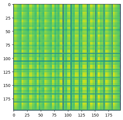
# Attention Matrix
attention_matrix = q @ kT
print("attention matrix: ", attention_matrix.shape)
plt.imshow(attention_matrix[3].detach().cpu().numpy())

The final step involves visualizing the attention maps.

# Visualize attention matrix
fig = plt.figure(figsize=(16, 8))
fig.suptitle("Attention Maps Across Heads", fontsize=24)
# fig.add_axes()
img = np.asarray(img)
ax = fig.add_subplot(2, 4, 1)
ax.imshow(img)
ax.axis('off')
for i in range(7):
    attn_heatmap = attention_matrix[i, 64, 1:].reshape((14, 14)).detach().cpu().numpy()
    ax = fig.add_subplot(2, 4, i+2)
    ax.imshow(attn_heatmap)
    ax.axis('off')

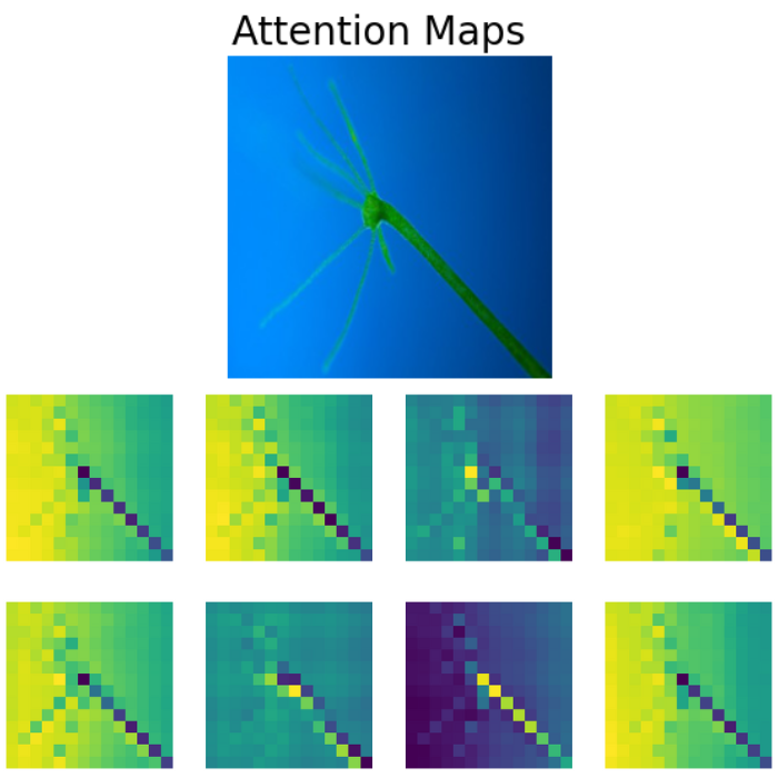
We can clearly see how the Vision Transformer model is attending to different parts of the Hydra. The Vision Transformer model is focusing on a different region in each of the images which makes Multi-Head Self Attention such a powerful technique.

Summary and Conclusion

We dived into fine tuning and visualizing attention maps of Vision Transformers in this article. We started with a basic discussion of the dataset, got into the training of the model, and visualized how the Vision Transformer model attends to different parts of an image. Although we did not get into the theoretical concepts here, I hope this article is useful to you.

If you have any doubts, thoughts, or suggestions, please leave them in the comment section. I will surely address them.

You can contact me using the Contact section. You can also find me on LinkedIn, and Twitter.