Malaria Classification with Vision Transformer and PyTorch

In this article, we are going to carry out malaria classification with vision transformer and PyTorch. While malaria can be detected from blood samples and laboratory testing, we can speed up the process using deep learning and computer vision. Malaria can be life-threatening if not diagnosed on time. With deep learning, we can train an image classification model that can recognize whether a zoomed-in blood-smear sample has malaria parasites or not. For this malaria classification model, we will employ a vision transformer and the PyTorch framework.

Note that 5 plasmodium species cause malaria in humans. However, in this article, we will classify whether a blood sample contains a malarial parasite or not. We will not distinguish between the different species of Plasmodium. This is just getting started with malaria classification with vision transformer, so, we keep the problem statement simple.

We will cover the following points here:

• We will start with a discussion of the malaria classification dataset.
• Next, we will move on to discuss the codebase that we will use to train the vision transformer model on the dataset.
• After training, we will prepare a notebook to run testing, inference, and visualizing attention maps.
• We will end the article with prospects and points for improvement.

The Malaria Classification Dataset

We will train the vision transformer model on the BioImage Informatics II Malaria Dataset available on Kaggle.

The dataset contains a train and a test folder with the class folders in each of them. There are two classes: parasitized and uninfected. Here is the dataset structure:

├── test
│   ├── parasitized
│   └── uninfected
└── train
    ├── parasitized
    └── uninfected

The train folder contains 10900 samples for the parasitized and 11000 samples for the uninfected classes. Similarly, for the test set, the sample count is 3571 for the parasitized and 3572 for the uninfected class.

We will divide the current training set into a training and validation set and keep the test set aside for running evaluation.

Here are a few samples from the dataset.

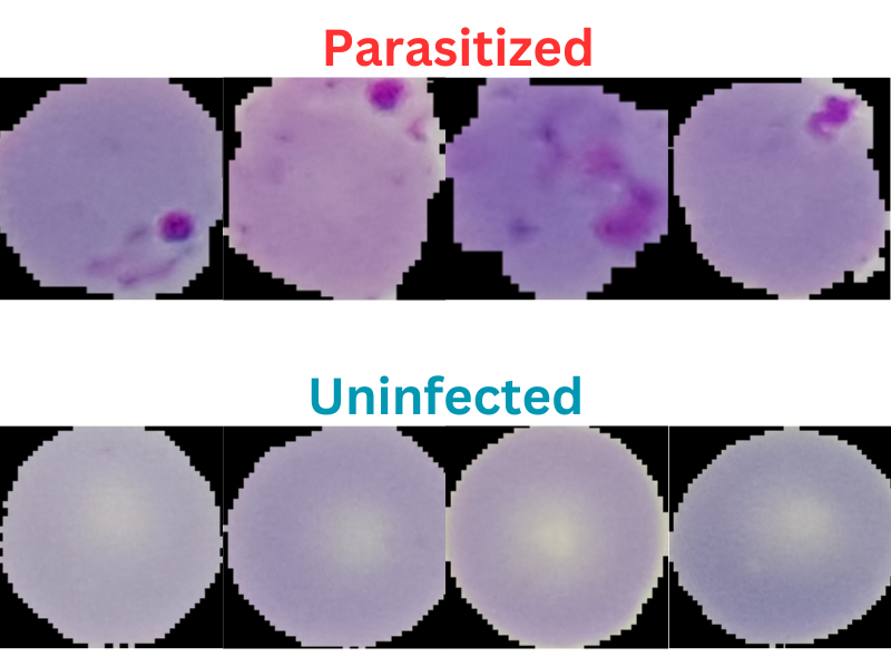
As we can see, the dataset does not seem that much challenging. This is mainly because the blood smear samples are already cropped to a center region where the parasite may be present. Still, we will train as good a model as we can and see how it performs.

As we already discussed, this is an easy problem for an image classification model, and we will cover a much more comprehensive and difficult one in a future article.

The Vision Transformer Codebase and Setup

We will use a modified version of the vision_transformers library that I actively maintain. You don’t need to clone it. Instead, all the code is available for download via the download section of this article. This will ensure that future updates to the repository do not break the code in this article.

Download Code

After downloading the code, extract it and enter the src directory.

First, install PyTorch with CUDA. The following commands are expected to be executed in an Anaconda environment.

conda install pytorch torchvision torchaudio pytorch-cuda=11.7 -c pytorch -c nvidia

Then install the library.

pip install .

This will let us import the vision_transformers library from wherever we want.

Next, install the requirements.

pip install -r requirements.txt

With this, we are done with all the setup we need.

Final Project Directory Structure

The following block shows the final project directory.

├── input
│   └── dataset
│       ├── test
│       └── train
└── src
    ├── build
    ├── data
    ├── examples
    ├── example_test_data
    ├── readme_images
    ├── runs
    │   └── training
    ├── tools
    ├── vision_transformers
    ├── vision_transformers.egg-info
    ├── inference.ipynb
    ├── README.md
    ├── requirements.txt
    └── setup.py

• The input directory contains the malaria classification dataset that we will use for training the vision transformer model.
• The src directory contains all the code we need for training, testing, and inference. We also have an inference.ipynb file that contains the code for inference and visualization of attention maps.

The pretrained weights are available through the downloadable zip file. They are present inside src/runs/training/vit_ti_5e_128b directory. You can directly jump to the inference section in case you do not intend to train the model. If you are planning to train the model, download the dataset and set it up according to the above directory structure.

Malaria Classification with Vision Transformer

In this section, we will go through the technical and coding aspects of the article. This will include the dataset preparation and training. Do note that we will not go through the details of the model architecture before training. As the codebase is part of a library, it is quite large. However, we will go through the steps that are absolutely necessary.

The ViT Tiny Model

For training on the malaria classification dataset, we will use the ViT Tiny model. In the library, we refer to this model as vit_ti_p16_224. The naming convention lets us know that the ViT Tiny model converts each 224×224 image into 16×16 patches. As the dataset is quite simple, we do not need to use any larger model right away. The model has been pretrained on the ImageNet weights.

For 2 classes, the final model contains roughly 5.5 million parameters. Compared to the base ViT, the ViT Tiny model has a smaller embedding layer. It contains a 192-dimensional embedding instead of a 768-dimensional embedding.

The following image shows the compact architecture from the terminal output after the initialization of the entire model.

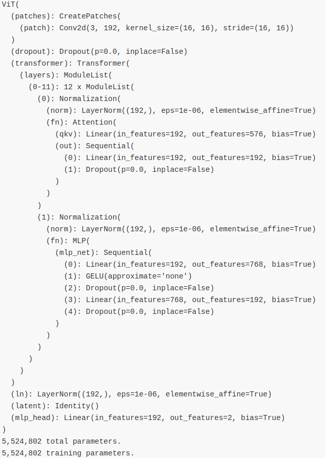
The ViT Tiny model contains 12 transformer layers just like the base model.

Dataset and Data Loader

As we are using ImageNet pretrained weights, the images pass through ImageNet normalization values. Further, each image gets resized to 224×224 resolution. These processes are the same for both, the training and the validation data loaders.

For training, we do not apply any data augmentations right away. However, you may go into tools/utils/transforms.py and modify the get_train_transform() function to add augmentations.

Note: You do not need to reinstall the library in case you make changes in the tools directory.

Training the ViT Tiny Model on the Malaria Classification Dataset

All the training experiments were done on a machine with 10 GB RTX 3080 GPU, 10th generation i7 CPU, and 32 GB of RAM.

The codebase contains a train_classifier.py file for image classification using Vision Transformers. We just need to execute the script with the necessary arguments to start the training.

To start the training, we need to execute the following command within the src directory. We are not training the vision transformer model from scratch. Executing the command the first time will download and load the pretrained weights.

python tools/train_classifier.py --data ../input/dataset/train 0.15 --epochs 5 --model vit_ti_p16_224 --learning-rate 0.0005 --batch 128 --name vit_ti_5e_128b

Let’s go through the command line arguments that we are using above:

• --data: This is the path to the dataset directory. The data needs to be in PyTorch ImageFolder format where all the images should be in their respective class folders. This argument takes multiple values. As we want to split the data in this directory into a training and validation set, after providing the path we also provide the ratio for the validation set. Here, we are using 15% of the data for validation.
• --epochs: The number of epochs to train for.
• --model: This is the model that we want to train. Here, we provide vit_ti_p16_224 to train the ViT Tiny model. Please take a look inside vision_transformers/models/vit.py file to check all the available models.
• --learning-rate: The initial learning rate. We start with a learning rate of 0.0005.
• --batch: The batch size for the data loaders. You may reduce the batch size in case you face Out Of Memory error.
• --name: This is the folder name where all the results are saved. This folder will be present inside runs/training directory.

As we are using the tiny model, the training will be over within a few minutes.

Analyzing the Training Results

The following block shows the truncated output from the terminal.

[INFO]: Epoch 1 of 5
Training
100%|████████████████████████████████████████████████████████████████████████████████████████████████████████████████████████████████████████████████████████████████████████████| 146/146 [00:20<00:00,  7.17it/s]
Validation
100%|██████████████████████████████████████████████████████████████████████████████████████████████████████████████████████████████████████████████████████████████████████████████| 26/26 [00:01<00:00, 14.59it/s]

LOWEST VALIDATION LOSS: 0.10308248692980179

SAVING BEST MODEL FOR EPOCH: 1

SAVING PLOTS COMPLETE...
Training loss: 0.182, training acc: 93.928
Validation loss: 0.103, validation acc: 96.312
--------------------------------------------------
[INFO]: Epoch 5 of 5
Training
100%|████████████████████████████████████████████████████████████████████████████████████████████████████████████████████████████████████████████████████████████████████████████| 146/146 [00:18<00:00,  7.73it/s]
Validation
100%|██████████████████████████████████████████████████████████████████████████████████████████████████████████████████████████████████████████████████████████████████████████████| 26/26 [00:01<00:00, 14.68it/s]

LOWEST VALIDATION LOSS: 0.09319936856627464

SAVING BEST MODEL FOR EPOCH: 5

SAVING PLOTS COMPLETE...
Training loss: 0.068, training acc: 97.392
Validation loss: 0.093, validation acc: 97.044
--------------------------------------------------
TRAINING COMPLETE

The model already reaches 97% validation accuracy on epoch 5. This is also the best accuracy. The validation loss is 0.093 which is the least loss as well. We will use the model from the last epoch for inference and evaluation.

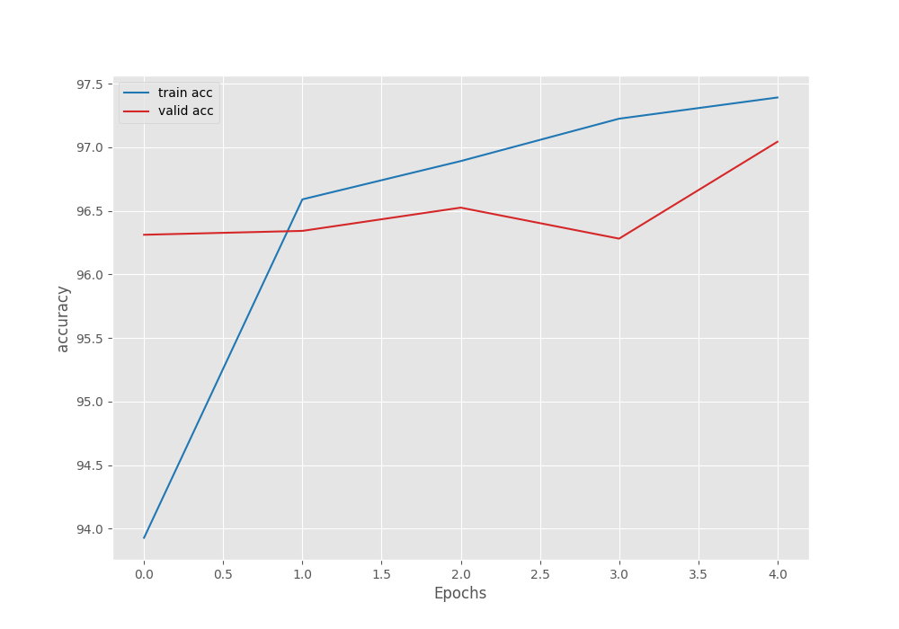
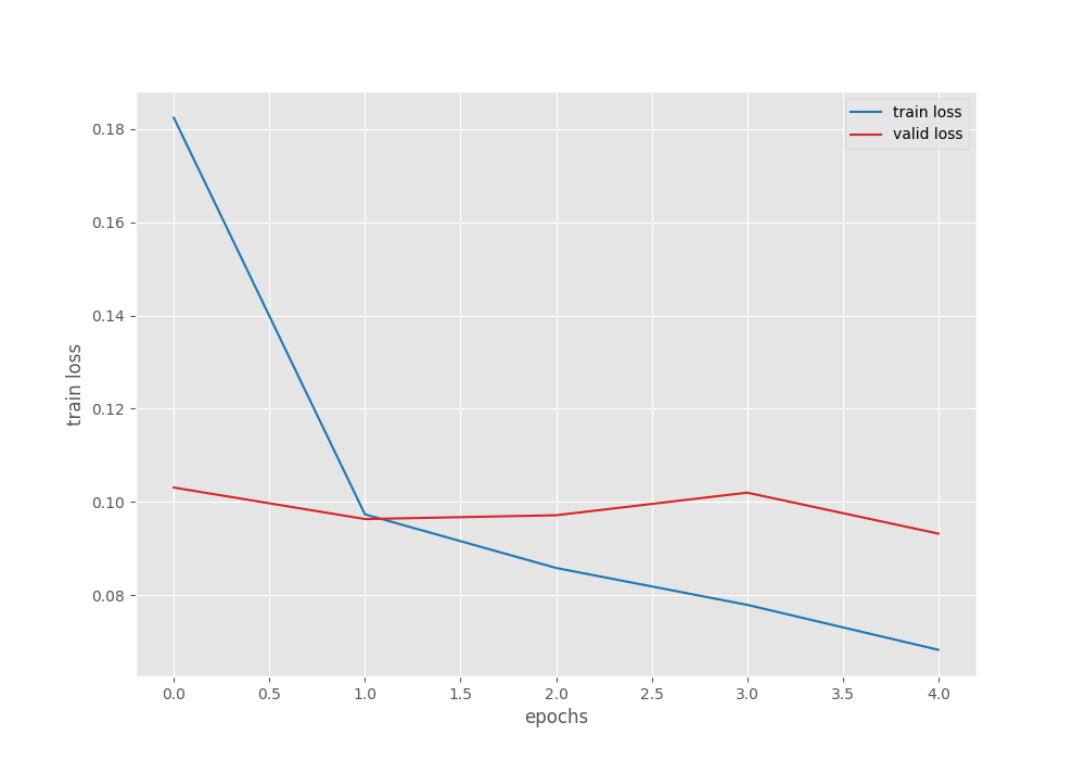
From the graphs, it is clear that we could have trained for a few more epochs to get even better results. For now, let’s move on to the inference and evaluation stage.

Inference, Evaluation, and Visualization of Attention Maps

All the code from here follows the inference.ipynb notebook present inside the src directory. The notebook accomplishes three tasks:

• It loads the pretrained model and runs inference on a few images from the test set.
• Then it evaluates the model on the test set to calculate the loss and accuracy.
• Finally, it computes the attention maps using the trained weights.

Let’s start. First, we need to import all the packages and libraries and define the computation device.

import torch
import torchvision.transforms as transforms
import numpy as np
import matplotlib.pyplot as plt
import glob
import torch.nn as nn

from PIL import Image
from vision_transformers.models import vit
from tools.utils.transforms import get_valid_transform
from torch.utils.data import DataLoader
from torchvision import datasets
from tqdm import tqdm

device = torch.device('cuda:0' if torch.cuda.is_available() else 'cpu')

Next, let’s create a list containing the class names. This will be useful during the inference stage.

class_names = [
    'parasitized',
    'uninfected'
]

Now, we need to initialize the model, load the trained weights, and define the transforms for the inference stage.

model = vit.vit_ti_p16_224(num_classes=len(class_names), pretrained=False).eval()
ckpt = torch.load('runs/training/vit_ti_5e_128b/best_model.pth')
model.load_state_dict(ckpt['model_state_dict'])

transform = transforms.Compose([
    transforms.ToTensor(),
    transforms.Normalize(
        mean = [0.485, 0.456, 0.406],
        std = [0.229, 0.224, 0.225]
    )
])

Inference

For running inference, the following code block defines a simple function. It takes in an image path, reads it, applies the necessary preprocessing, and forward passes it through the model.

def infer(image_path):
    image = Image.open(image_path)
    image = image.resize((224, 224))
    plt.figure(figsize=(6, 3))
    plt.imshow(image)
    plt.axis('off')
    input_tensor = transform(image).unsqueeze(0)
    with torch.no_grad():
        output = model(input_tensor)
    
    probabilities = torch.nn.functional.softmax(output[0], dim=0)
    probabilities = probabilities.numpy()
    category = class_names[np.argmax(probabilities)]
    plt.text(x=10, y=20, s=category, fontsize='large', color='red')
    plt.show()

First, let’s run inference on the test images in the parasitized folder. We break the inference loop after 10 images.

image_paths = glob.glob('../input/dataset/test/parasitized/*')
for i, image_path in enumerate(image_paths):
    if i == 10:
        break
    infer(image_path)

Here are the results.

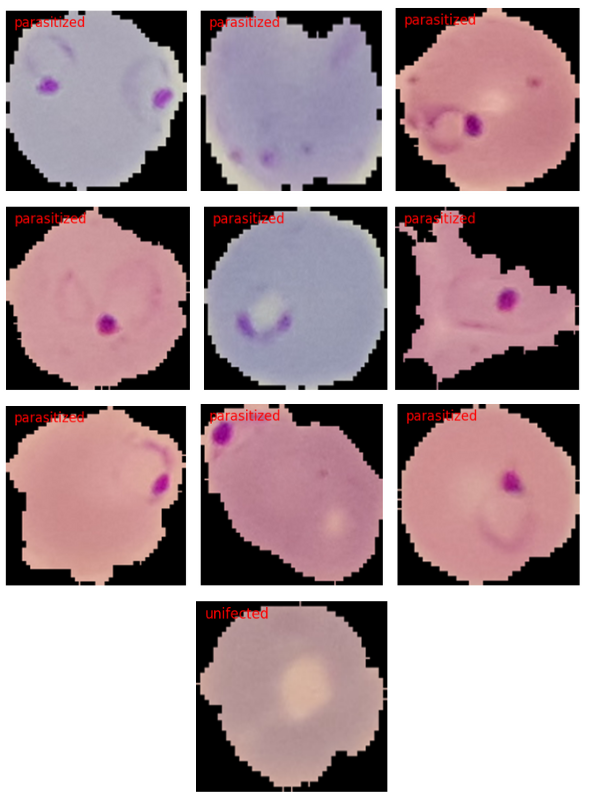
The model is able to predict the classes of 9 out of 10 images correctly.

Next, let’s run inference on the images from the uninfected folder.

image_paths = glob.glob('../input/dataset/test/parasitized/*')
for i, image_path in enumerate(image_paths):
    if i == 10:
        break
    infer(image_path)

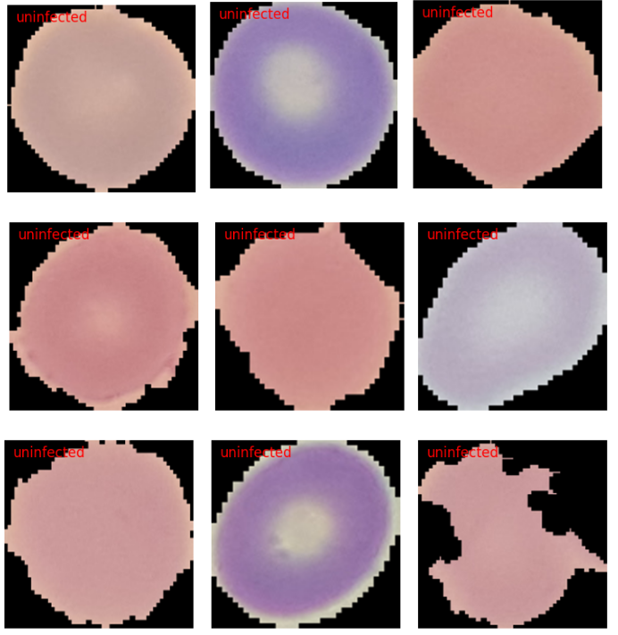
In this case, all the results are correct. However, visualizing a few more results may reveal some wrong predictions.

Evaluation on the Test Set

For evaluation, we take the following steps:

• Create the test dataset and data loader.
• Define the loss function.
• Create a validate() function that will carry out the evaluation.

# Create test dataset.
dataset_test = datasets.ImageFolder(
    '../input/dataset/test', 
    transform=(get_valid_transform(224))
)

print(f"Number of test samples: {len(dataset_test)}")

The above code block prints the number of samples in the test set which is 7143.

test_dataloader = DataLoader(
        dataset_test,
        batch_size=128,
        num_workers=4,
        shuffle=False
    )

# Loss function.
criterion = nn.CrossEntropyLoss()

def validate(model, testloader, criterion):
    model.eval().to(device)
    valid_running_loss = 0.0
    valid_running_correct = 0
    counter = 0

    with torch.no_grad():
        for i, data in tqdm(enumerate(testloader), total=len(testloader)):
            counter += 1
            
            image, labels = data
            image = image.to(device)
            labels = labels.to(device)
            # Forward pass.
            outputs = model(image)
            # Calculate the loss.
            loss = criterion(outputs, labels)
            valid_running_loss += loss.item()
            # Calculate the accuracy.
            _, preds = torch.max(outputs.data, 1)
            valid_running_correct += (preds == labels).sum().item()
        
    # Loss and accuracy for the complete epoch.
    epoch_loss = valid_running_loss / counter
    epoch_acc = 100. * (valid_running_correct / len(testloader.dataset))
    return epoch_loss, epoch_acc

Finally, call the validate() function with the appropriate arguments.

test_loss, test_acc = validate(model, test_dataloader, criterion)
print(f"Test loss: {test_loss:.3f}, test accuracy: {test_acc:.3f}")

We get a test accuracy of 96.878% and a test loss of 0.90. This is really good considering we trained the ViT Tiny model for just 5 epochs.

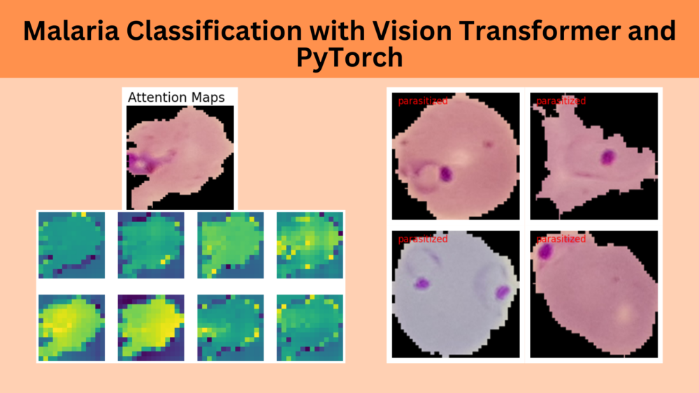
Visualizing Attention Maps

The final part of the article involves the visualization of the attention maps. This helps us understand where the vision transformer model is focusing while predicting a particular class.

In this section, we will not go through the theory of the code in detail. In case you want a detailed explanation, please go through the post where we fine tune vision transformer and visualize attention maps.

First, let’s load the model onto the CPU.

model = model.cpu()

Next, load an image containing the malaria parasite.

image = Image.open('../input/dataset/test/parasitized/C100P61ThinF_IMG_20150918_144823_cell_161.png')
image = image.resize((224, 224))
input_tensor = transform(image).unsqueeze(0)

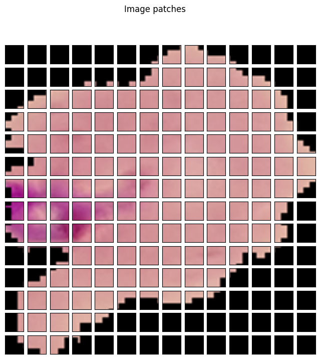
Then, we need to create patches from the image.

# Patch embedding.
patches = model.patches.patch(input_tensor)
print(f"Input tensor shape: {input_tensor.shape}")
print(f"Patch embedding shape: {patches.shape}")

This will create 14 patches of 16×16 resolution across the row and column. The following code block visualizes them.

fig = plt.figure(figsize=(8, 8))
fig.suptitle("Image patches", fontsize=12)
img = np.asarray(image)
for i in range(0, 196):
    x = i % 14
    y = i // 14
    patch = img[y*16:(y+1)*16, x*16:(x+1)*16]
    ax = fig.add_subplot(14, 14, i+1)
    ax.axes.get_xaxis().set_visible(False)
    ax.axes.get_yaxis().set_visible(False)
    ax.imshow(patch)

The next step is to get the positional embedding, reshape the patches, and find the input that will go into the transformer model.

pos_embed = model.pos_embedding
print(pos_embed.shape)

patch_input = patches.view(1, 192, 196).permute(0, 2, 1)
print(patch_input.shape)

transformer_input = torch.cat((model.cls_token, patch_input), dim=1) + pos_embed
print("Transformer input: ", transformer_input.shape)

Now, pass the input through the qkv layer of the model.

transformer_input_qkv = model.transformer.layers[0][0].fn.qkv(transformer_input)[0]
print(transformer_input_qkv.shape)

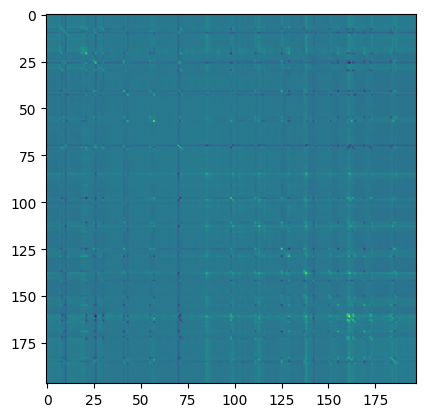
Next, compute the attention matrix.

qkv = transformer_input_qkv.reshape(197, 3, 12, 16)
print("Reshaped qkv : ", qkv.shape)
q = qkv[:, 0].permute(1, 0, 2)
k = qkv[:, 1].permute(1, 0, 2)
kT = k.permute(0, 2, 1)
print("K transposed: ", kT.shape)

# Attention Matrix
attention_matrix = q @ kT
print("Attention matrix: ", attention_matrix.shape)
plt.imshow(attention_matrix[3].detach().cpu().numpy())

Finally, visualize the attention maps.

# Visualize attention matrix
fig = plt.figure(figsize=(6, 3))
fig.suptitle("Attention Maps", fontsize=20)
# fig.add_axes()
img = np.asarray(img)
ax1 = fig.add_subplot(1, 1, 1)
ax1.imshow(img)
ax1.axis('off')
fig = plt.figure(figsize=(16, 8))
for i in range(8):
    attn_heatmap = attention_matrix[i, 64, 1:].reshape((14, 14)).detach().cpu().numpy()
    ax2 = fig.add_subplot(2, 4, i+1)
    ax2.imshow(attn_heatmap)
    ax2.axis('off')

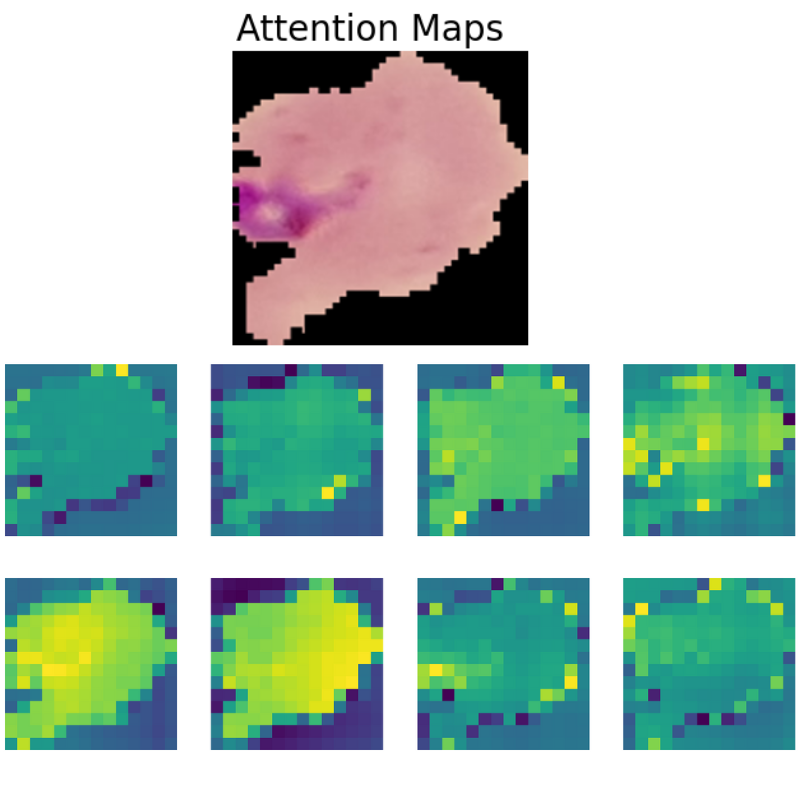
The attention maps make it clear how the model focuses on the areas where the malaria parasite is present. This shows how the model may predict a class when we provide it with an image.

Summary and Conclusion

In this article, we went through training a ViT Tiny model on a simple malaria classification dataset. As the dataset was easy to learn, the model was able to perform well within a few epochs of training only. Along with the classification results, we also visualized the attention maps of the model. This allowed us to analyze where the model was focusing when making predictions. In the next article, we will tackle a more difficult problem along the same line. I hope that this article was worth your time.

If you have any doubts, thoughts, or suggestions, please leave them in the comment section. I will surely address them.

You can contact me using the Contact section. You can also find me on LinkedIn, and Twitter.