Pretraining Faster RCNN ViT Detection Model on Pascal VOC

In deep learning, we mostly deal with fine-tuning, transfer learning, or creating solutions. These include training an already pretrained model on a new dataset till we get the desired results. However, we ignore the pretraining of the model almost entirely because of computing constraints. Most of the time, pretraining involves creating a model and training it on a sufficiently diverse dataset, like the COCO detection dataset. To reduce that knowledge gap, in this article, we will be pretraining a Faster RCNN ViT Detection model on the Pascal VOC dataset.

As of writing this, the Pascal VOC dataset is not considered a pretraining dataset most of the time. There are much larger datasets with hundreds of millions of images which give better pretrained models. So, why pretrain the Faster RCNN ViT Detection model on the Pascal VOC dataset?

• This is a good place to start to know how to deal with long training experiments.
• This will also give us the chance to create a new model by connecting different backbones and object detection modules in PyTorch. We will create a Faster RCNN object detection model with a Vision Transformer backbone.
• Finally, we will learn to deal with the intricacies of data preparation and data augmentation.

All in all, we will cover the following points in this article:

• We will start with a discussion of the Pascal VOC dataset.
• Then we will move on to the discussion of the codebase that we will use for training.
• Next, we will deal with the Faster RCNN ViT detection model preparation.
• We will follow this up with the pretraining experiments.
• After training, we will carry out inference on images and videos.
• Finally, we will discuss some points to further train the model to get even better results.

The Pascal VOC Dataset

Most of us already know about the Pascal VOC dataset. It remained an object detection benchmarking and pretraining dataset for a long time. With time, newer, larger datasets have taken its place. Even then, it remains a good dataset to experiment with and pretrain custom models with.

In this article, we will use the Pascal VOC dataset from Kaggle for pretraining the Faster RCNN ViT detection model.

The dataset that we will use already contains the 2012 and 2007 Pascal VOC combined sets. The preparation methodology followed the official text files for splitting the images year-wise. The annotations are present in XML format.

It contains 20 object classes. They are: “aeroplane”, “bicycle”, “bird”, “boat”, “bottle”, “bus”, “car”, “cat”, “chair”, “cow”, “diningtable”, “dog”, “horse”, “motorbike”, “person”, “pottedplant”, “sheep”, “sofa”, “train”, “tvmonitor”.

After downloading and extracting the dataset, we get the following structure.

voc_07_12/
└── final_xml_dataset
    ├── train
    │   ├── images
    │   └── labels
    └── valid
        ├── images
        └── labels

The images folders contain the images and labels folders contain the annotations files in XML format.

There are around 16600 training samples and 4950 validation samples in the combined Pascal VOC dataset. Here are a few images with the ground truth annotations from the dataset.

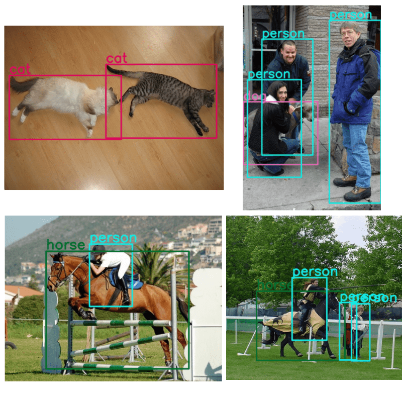
As we can see, the dataset is quite diverse. There are several objects in various scenes. This also gives us an idea of why the Pascal VOC dataset remained so prominent for so long.

The Faster RCNN PyTorch Training Pipeline

For the pretraining, we will use the Faster RCNN PyTorch Training pipeline. We have used this repository in previous posts to get excellent results using different Faster RCNN models.

Download Code

The codebase includes models like COCO pretrained Faster RCNN ResNet50 FPN V2 and many custom models as well. In fact, you can add any model you like by just combining different modules from PyTorch.

For this article, you need not clone the repository. The entire codebase is available via the download section. This ensures that future updates to the codebase do not break the commands in this article.

However, feel free to clone the repository as well and try some experiments like fine tuning the Faster RCNN ResNet50 FPN V2 model.

For now, after downloading and extracting the codebase from the download section, carry out the following steps to set everything in a new Anaconda environment:

• Enter the Faster RCNN training pipeline folder.

cd fasterrcnn-pytorch-training-pipeline

• Install PyTorch and Torchvision with CUDA support.

conda install pytorch torchvision torchaudio pytorch-cuda=11.7 -c pytorch -c nvidia

• Install the rest of the requirements.

pip install -r requirements.txt

That’s it, we are all set with the codebase.

The Project Directory Structure

Next, let’s take a look at the entire project directory structure.

├── fasterrcnn-pytorch-training-pipeline
│   ├── data
│   ├── data_configs
│   ├── docs
│   ├── example_test_data
│   ├── models
│   ├── notebook_examples
│   ├── readme_images
│   ├── torch_utils
│   ├── utils
│   ├── _config.yml
│   ├── datasets.py
│   ├── eval.py
│   ├── export.py
│   ├── inference.py
│   ├── inference_video.py
│   ├── __init__.py
│   ├── LICENSE
│   ├── onnx_inference_image.py
│   ├── onnx_inference_video.py
│   ├── README.md
│   ├── requirements.txt
│   └── train.py
└── input
    ├── inference_data
    └── voc_07_12

• The fasterrcnn-pytorch-training-pipeline contains all the code that we need for training the Faster RCNN ViT Detection model.
• The input directory contains all the data related files. This includes the voc_07_12 folder with the training dataset as we saw earlier. The inference_data directory contains data for running inference after training the model.

The best trained model weights and the inference data are present in the downloadable zip file. The trained weights are present in fasterrcnn-pytorch-training-pipeline/outputs/training/fasterrcnn_vitdet_voc directory. If you wish to run the training, you can download the dataset from the Kaggle link.

Pretraining Faster RCNN ViT Detection Model

Let’s get into the technical aspects of the article now. Although we will not be able to cover the entire codebase, we will discuss some of the most important parts. The most important of them is the Faster RCNN ViT detection model.

Other than that, we also discuss the augmentations that we apply to the dataset.

The Faster RCNN ViT Detection Model

All the model code for the library are present in the models directory. As of writing this, 28 models are present in the library. All of them are Faster RCNN based. Some are pretrained ones and some are not, though we will not focus on that much here.

The fasterrcnn_vitdet.py contains the code that we are interested in. We will only discuss the components present in this Python file. It imports several helper functions and classes from the layers.py file in the same directory. However, we cannot discuss that here as it is more than 700 lines of code.

A lot of code has been adapted from the Detectron2 codebase. For example, the backbone that we use here is a Vision Transformer Base model with Masked Autoencoder. We use pretrained backbones to get a headstart.

First, let’s import all the modules and packages.

import torch.nn as nn
import torch
import torch.nn.functional as F
import math
import torchvision

from functools import partial
from torchvision.models.detection import FasterRCNN
from models.layers import (
    Backbone, 
    PatchEmbed, 
    Block, 
    get_abs_pos,
    get_norm,
    Conv2d,
    LastLevelMaxPool
)
from models.utils import _assert_strides_are_log2_contiguous

We import the FasterRCNN from Torchvision as that’s what we need to build the final detection model after combining all the components.

As we discussed before, layers module contains a lot of helper functions and classes. Most of these help with the proper building of the backbone.

The Vision Transformer Backbone

The Vision Transformer backbone that we use to build the Faster RCNN ViT Detection model is almost the same as described in the paper. However, minor changes have been made so that it be easily combined with a detection head. The following code block contains the entire ViT class.

class ViT(Backbone):
    """
    This module implements Vision Transformer (ViT) backbone in :paper:`vitdet`.
    "Exploring Plain Vision Transformer Backbones for Object Detection",
    https://arxiv.org/abs/2203.16527
    """

    def __init__(
        self,
        img_size=1024,
        patch_size=16,
        in_chans=3,
        embed_dim=768,
        depth=12,
        num_heads=12,
        mlp_ratio=4.0,
        qkv_bias=True,
        drop_path_rate=0.0,
        norm_layer=nn.LayerNorm,
        act_layer=nn.GELU,
        use_abs_pos=True,
        use_rel_pos=False,
        rel_pos_zero_init=True,
        window_size=0,
        window_block_indexes=(),
        residual_block_indexes=(),
        use_act_checkpoint=False,
        pretrain_img_size=224,
        pretrain_use_cls_token=True,
        out_feature="last_feat",
    ):
        """
        
        :param img_size (int): Input image size.
        :param patch_size (int): Patch size.
        :param in_chans (int): Number of input image channels.
        :param embed_dim (int): Patch embedding dimension.
        :param depth (int): Depth of ViT.
        :param num_heads (int): Number of attention heads in each ViT block.
        :param mlp_ratio (float): Ratio of mlp hidden dim to embedding dim.
        :param qkv_bias (bool): If True, add a learnable bias to query, key, value.
        :param drop_path_rate (float): Stochastic depth rate.
        :param norm_layer (nn.Module): Normalization layer.
        :param act_layer (nn.Module): Activation layer.
        :param use_abs_pos (bool): If True, use absolute positional embeddings.
        :param use_rel_pos (bool): If True, add relative positional embeddings to the attention map.
        :param rel_pos_zero_init (bool): If True, zero initialize relative positional parameters.
        :param window_size (int): Window size for window attention blocks.
        :param window_block_indexes (list): Indexes for blocks using window attention.
        :param residual_block_indexes (list): Indexes for blocks using conv propagation.
        :param use_act_checkpoint (bool): If True, use activation checkpointing.
        :param pretrain_img_size (int): input image size for pretraining models.
        :param pretrain_use_cls_token (bool): If True, pretrainig models use class token.
        :param out_feature (str): name of the feature from the last block.
        """
        super().__init__()
        self.pretrain_use_cls_token = pretrain_use_cls_token

        self.patch_embed = PatchEmbed(
            kernel_size=(patch_size, patch_size),
            stride=(patch_size, patch_size),
            in_chans=in_chans,
            embed_dim=embed_dim,
        )

        if use_abs_pos:
            # Initialize absolute positional embedding with pretrain image size.
            num_patches = (pretrain_img_size // patch_size) * (pretrain_img_size // patch_size)
            num_positions = (num_patches + 1) if pretrain_use_cls_token else num_patches
            self.pos_embed = nn.Parameter(torch.zeros(1, num_positions, embed_dim))
        else:
            self.pos_embed = None

        # stochastic depth decay rule
        dpr = [x.item() for x in torch.linspace(0, drop_path_rate, depth)]

        self.blocks = nn.ModuleList()
        for i in range(depth):
            block = Block(
                dim=embed_dim,
                num_heads=num_heads,
                mlp_ratio=mlp_ratio,
                qkv_bias=qkv_bias,
                drop_path=dpr[i],
                norm_layer=norm_layer,
                act_layer=act_layer,
                use_rel_pos=use_rel_pos,
                rel_pos_zero_init=rel_pos_zero_init,
                window_size=window_size if i in window_block_indexes else 0,
                use_residual_block=i in residual_block_indexes,
                input_size=(img_size // patch_size, img_size // patch_size),
            )
            if use_act_checkpoint:
                # TODO: use torch.utils.checkpoint
                from fairscale.nn.checkpoint import checkpoint_wrapper

                block = checkpoint_wrapper(block)
            self.blocks.append(block)

        self._out_feature_channels = {out_feature: embed_dim}
        self._out_feature_strides = {out_feature: patch_size}
        self._out_features = [out_feature]

        if self.pos_embed is not None:
            nn.init.trunc_normal_(self.pos_embed, std=0.02)

        self.apply(self._init_weights)

    def _init_weights(self, m):
        if isinstance(m, nn.Linear):
            nn.init.trunc_normal_(m.weight, std=0.02)
            if isinstance(m, nn.Linear) and m.bias is not None:
                nn.init.constant_(m.bias, 0)
        elif isinstance(m, nn.LayerNorm):
            nn.init.constant_(m.bias, 0)
            nn.init.constant_(m.weight, 1.0)

    def forward(self, x):
        x = self.patch_embed(x)
        if self.pos_embed is not None:
            x = x + get_abs_pos(
                self.pos_embed, self.pretrain_use_cls_token, (x.shape[1], x.shape[2])
            )

        for blk in self.blocks:
            x = blk(x)

        outputs = {self._out_features[0]: x.permute(0, 3, 1, 2)}
        return outputs

It follows the same initial approach as any other ViT. First, it creates patches, then the positional embeddings (lines 77 to 90).

Just like the ViT Base model, this backbone also contains 12 Transformer layers. The Transformer blocks get built using the Block class starting from line 97.

The Feature Pyramid Block

We also need a Feature Pyramid block for better performance of the model. The ViTDet paper introduces a SimpleFeaturePyramid class the proves to be essential when dealing with Vision Transformer based backbones and building detection models.

class SimpleFeaturePyramid(Backbone):
    """
    This module implements SimpleFeaturePyramid in :paper:`vitdet`.
    It creates pyramid features built on top of the input feature map.
    """

    def __init__(
        self,
        net,
        in_feature,
        out_channels,
        scale_factors,
        top_block=None,
        norm="LN",
        square_pad=0,
    ):
        """
        :param net (Backbone): module representing the subnetwork backbone.
                Must be a subclass of :class:`Backbone`.
        :param in_feature (str): names of the input feature maps coming
                from the net.
        :param out_channels (int): number of channels in the output feature maps.
        :param scale_factors (list[float]): list of scaling factors to upsample or downsample
                the input features for creating pyramid features.
        :param top_block (nn.Module or None): if provided, an extra operation will
                be performed on the output of the last (smallest resolution)
                pyramid output, and the result will extend the result list. The top_block
                further downsamples the feature map. It must have an attribute
                "num_levels", meaning the number of extra pyramid levels added by
                this block, and "in_feature", which is a string representing
                its input feature (e.g., p5).
        :param norm (str): the normalization to use.
        :param square_pad (int): If > 0, require input images to be padded to specific square size.
        """
        super(SimpleFeaturePyramid, self).__init__()
        assert isinstance(net, Backbone)

        self.scale_factors = scale_factors

        input_shapes = net.output_shape()
        strides = [int(input_shapes[in_feature].stride / scale) for scale in scale_factors]
        _assert_strides_are_log2_contiguous(strides)

        dim = input_shapes[in_feature].channels
        self.stages = []
        use_bias = norm == ""
        for idx, scale in enumerate(scale_factors):
            out_dim = dim
            if scale == 4.0:
                layers = [
                    nn.ConvTranspose2d(dim, dim // 2, kernel_size=2, stride=2),
                    get_norm(norm, dim // 2),
                    nn.GELU(),
                    nn.ConvTranspose2d(dim // 2, dim // 4, kernel_size=2, stride=2),
                ]
                out_dim = dim // 4
            elif scale == 2.0:
                layers = [nn.ConvTranspose2d(dim, dim // 2, kernel_size=2, stride=2)]
                out_dim = dim // 2
            elif scale == 1.0:
                layers = []
            elif scale == 0.5:
                layers = [nn.MaxPool2d(kernel_size=2, stride=2)]
            else:
                raise NotImplementedError(f"scale_factor={scale} is not supported yet.")

            layers.extend(
                [
                    Conv2d(
                        out_dim,
                        out_channels,
                        kernel_size=1,
                        bias=use_bias,
                        norm=get_norm(norm, out_channels),
                    ),
                    Conv2d(
                        out_channels,
                        out_channels,
                        kernel_size=3,
                        padding=1,
                        bias=use_bias,
                        norm=get_norm(norm, out_channels),
                    ),
                ]
            )
            layers = nn.Sequential(*layers)

            stage = int(math.log2(strides[idx]))
            self.add_module(f"simfp_{stage}", layers)
            self.stages.append(layers)

        self.net = net
        self.in_feature = in_feature
        self.top_block = top_block
        # Return feature names are "p<stage>", like ["p2", "p3", ..., "p6"]
        self._out_feature_strides = {"p{}".format(int(math.log2(s))): s for s in strides}
        # top block output feature maps.
        if self.top_block is not None:
            for s in range(stage, stage + self.top_block.num_levels):
                self._out_feature_strides["p{}".format(s + 1)] = 2 ** (s + 1)

        self._out_features = list(self._out_feature_strides.keys())
        self._out_feature_channels = {k: out_channels for k in self._out_features}
        self._size_divisibility = strides[-1]
        self._square_pad = square_pad

    @property
    def padding_constraints(self):
        return {
            "size_divisiblity": self._size_divisibility,
            "square_size": self._square_pad,
        }

    def forward(self, x):
        """
        :param x: Tensor of shape (N,C,H,W). H, W must be a multiple of ``self.size_divisibility``.
        Returns:
            dict[str->Tensor]:
                mapping from feature map name to pyramid feature map tensor
                in high to low resolution order. Returned feature names follow the FPN
                convention: "p<stage>", where stage has stride = 2 ** stage e.g.,
                ["p2", "p3", ..., "p6"].
        """
        bottom_up_features = self.net(x)
        features = bottom_up_features[self.in_feature]
        results = []

        for stage in self.stages:
            results.append(stage(features))

        if self.top_block is not None:
            if self.top_block.in_feature in bottom_up_features:
                top_block_in_feature = bottom_up_features[self.top_block.in_feature]
            else:
                top_block_in_feature = results[self._out_features.index(self.top_block.in_feature)]
            results.extend(self.top_block(top_block_in_feature))
        assert len(self._out_features) == len(results)
        return {f: res for f, res in zip(self._out_features, results)} 

There are of course a lot of things going in the above code block. Simply put:

• The SimpleFeaturePyramid class accepts the ViT backbone (net) as one of the parameters with several others.
• It also creates 2D convolutional stages for Feature Pyramid connections (lines 214 to 237).
• In the forward() method, first, it extracts the ViT Base features and then creates the Feature Pyramid connections (lines 271 to 276).

The Final VitDet Model

For the final ViTDet model, we will create a create_model() function.

def create_model(num_classes=81, pretrained=True, coco_model=False):
    # Base
    embed_dim, depth, num_heads, dp = 768, 12, 12, 0.1
    # Load the pretrained SqueezeNet1_1 backbone.
    net = ViT(  # Single-scale ViT backbone
        img_size=1024,
        patch_size=16,
        embed_dim=embed_dim,
        depth=depth,
        num_heads=num_heads,
        drop_path_rate=dp,
        window_size=14,
        mlp_ratio=4,
        qkv_bias=True,
        norm_layer=partial(nn.LayerNorm, eps=1e-6),
        window_block_indexes=[
            # 2, 5, 8 11 for global attention
            0,
            1,
            3,
            4,
            6,
            7,
            9,
            10,
        ],
        residual_block_indexes=[],
        use_rel_pos=True,
        out_feature="last_feat",
    )

    if pretrained:
        print('Loading MAE Pretrained ViT Base weights...')
        # ckpt = torch.utis('weights/mae_pretrain_vit_base.pth')
        ckpt = torch.hub.load_state_dict_from_url('https://dl.fbaipublicfiles.com/mae/pretrain/mae_pretrain_vit_base.pth')
        net.load_state_dict(ckpt['model'], strict=False)

    backbone = SimpleFeaturePyramid(
        net,
        in_feature="last_feat",
        out_channels=256,
        scale_factors=(4.0, 2.0, 1.0, 0.5),
        top_block=LastLevelMaxPool(),
        norm="LN",
        square_pad=1024,
    )

    backbone.out_channels = 256

    # Feature maps to perform RoI cropping.
    # If backbone returns a Tensor, `featmap_names` is expected to
    # be [0]. We can choose which feature maps to use.
    roi_pooler = torchvision.ops.MultiScaleRoIAlign(
        featmap_names=backbone._out_features,
        output_size=7,
        sampling_ratio=2
    )

    # Final Faster RCNN model.
    model = FasterRCNN(
        backbone=backbone,
        num_classes=num_classes,
        box_roi_pool=roi_pooler
    )
    return model

if __name__ == '__main__':
    from model_summary import summary
    model = create_model(81, pretrained=True)
    summary(model)

The above block carries out the following steps to create the Faster RCNN ViT Detection model:

• It first defines the embedding dimensions, the model depth (Transformer layers), the number of attention heads, and the dropout rate.
• Then it creates the ViT Base backbone which is stored in the net variable.
• Next, it loads the pretrained weights into the backbone. These are the official Masked Autoencoder based Vision Transformer Base model weights. The model was pretrained on the ImageNet1K dataset.
• Then we create the final backbone by employing the Feature Pyramid Network and passing the ViT Base model to it.
• The number of output channels from the backbone is 256 which is passed while defining the Feature Pyramid Network.
• Then we create the Region of Interest network (roi_pooler) which is an essential part of the Faster RCNN Model.
• Finally, we define the model by initializing the FasterRCNN model with the backbone, number of classes, and the Region of Interest Pooler.

The final model with 21 classes (20 Pascal VOC classes and one background class) contains around 101 million parameters. It is not that small a model after all.

Preparing the Pascal VOC Dataset and Data Augmentations

The Pascal VOC dataset contains the annotations in XML format already. So, we do not have to do much processing on that front.

While training the model, we will apply a lot of image augmentations using Albumentations. These include:

• Either one of Blur, Motion Blur, or Median Blur
• Randomly converting images to grayscale
• Randomly changing the color, brightness, and contrast
• And randomly changing the gamma

Albumentations helps in handling the bounding box augmentation along with the image augmentation.

The above augmentations prevent overfitting and also add a good amount of variation to the dataset. Following are some examples of images after applying the augmentations.

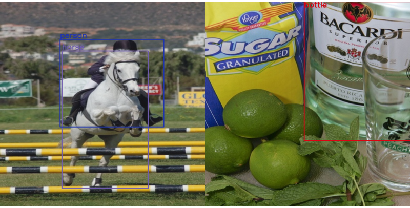
We are done with the dataset preparation here.

Training the Faster RCNN ViTDet Model on the Pascal VOC Dataset

Let’s get down to the interesting stuff, training the model.

All training and inference experiments were done on a machine with 10 GB RTX 3080 GPU, 10th generation i7 CPU, and 32 GB of RAM.

Execute the following command within the fasterrcnn-pytorch-training-pipeline to start the training.

python train.py --model fasterrcnn_vitdet --data data_configs/voc.yaml --epochs 50 --batch 2 --imgsz 640 --square-training --use-train-aug --name fasterrcnn_vitdet_voc --lr 0.005

Let’s go over the training arguments.

• --model: This is the model that we want to train. You can find all the supported trainable models inside models/__init__.py.
• --data: This is the path to the dataset YAML file. It contains the path to the images and annotation files along with the class names.
• --epochs: The number of epochs that we want to train the model for.
• --batch: The batch size for the data loader.
• --imgsz: This is the image size. As the next argument is --square-training, so, the width and height will be resized to 640 resolution each.
• --use-train-aug: This is a boolean argument telling the training pipeline to apply the augmentations that we discussed in the previous section.
• --name: The resulting project directory name.
• --lr: The learning rate for the optimizer.

The training may take a long time depending on the hardware. For comparison, on the mentioned system, each training epoch took around 39 minutes and an additional 3 minutes for each validation epoch.

The training was stopped after 32 epochs as the evaluation mAP metrics had stopped improving. Here are the mAP graphs.

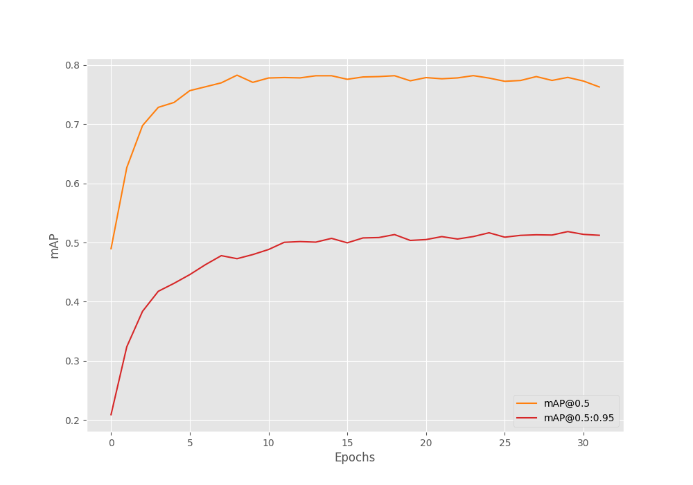
We can see the graphs started going down after epoch 31.

Till this point, we have the best mAP of 51.8% on epochs 30. Of course, there are a lot of other ways to keep improving the metric and training longer, but we will move forward with the current model.

Running Inference using Pretrained Faster RCNN ViTDet Model

Let’s start with running inference on images using the inference.py script. All the inference data are available inside the input/inference_data directory and come with the downloadable zip file.

python inference.py --weights outputs/training/fasterrcnn_vitdet_voc/best_model.pth --input ../input/inference_data/ --imgsz 640 --square-img --threshold 0.90

• The --weights argument takes a path to the model weight file that we want. We are using the best model weights.
• We provide the path to the input directory using the --input argument. This will run inference on all the images inside the directory.
• The image size is 640 as that’s what we trained on. Also, we are passing --square-img so that the script will resize the images to 640×640. This matches the training setting to get the best results.
• The detection threshold (--threshold) is 90%.

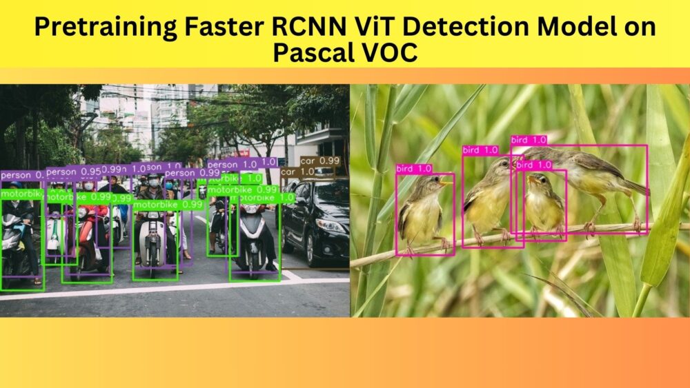
Here are the results.

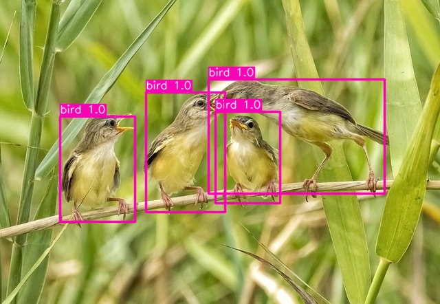
In the first image, the model is detecting all the birds with 100% confidence.

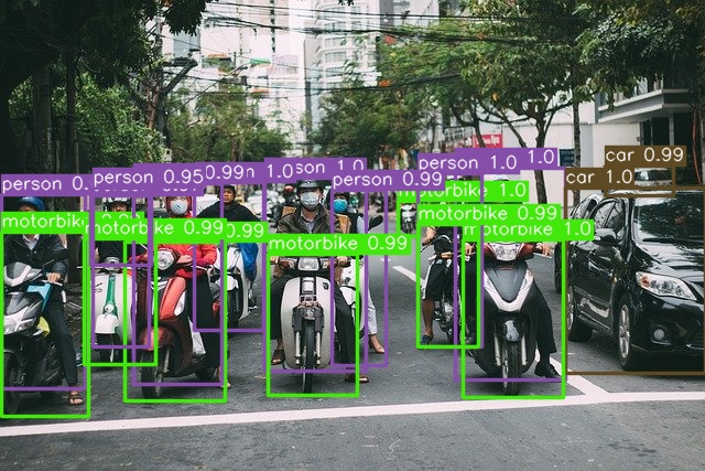
In the second image, along with all the people and motorbike, it is even able to detect the car at the far back.

Now, let’s move on to running inference on a video. We will use the inference_video.py script for this.

python inference_video.py --weights outputs/training/fasterrcnn_vitdet_voc/best_model.pth --input ../input/inference_data/video_1.mp4 --imgsz 640 --square-img --threshold 0.90

We can also add the --show argument at the end to visualize the result in real-time on screen.

Following is the resulting video.

The results are very good. Almost all the objects are detected with very high confidence. In fact, the model is even able to differentiate between bicycles and motorbikes which indicates that we have a really well trained model.

Further Improvements

We do not need to stop experimenting here. We have the best model. Why not continue training the model? We can next continue training with mosaic augmentation to make the model even better at handling small objects and occlusions. Take a look at the repository in case you are interested in running training with mosaic augmentation.

Summary and Conclusion

In this article, we went through the process of pretraining the Faster RCNN ViT Detection on the Pascal VOC dataset. Along the way, we saw how to prepare the Faster RCNN ViTDet model, how to arrange a large code library, and also what type of augmentations to use to prevent overfitting. This also led to the realization that pretraining object detection models can be time consuming and costly. Each training epoch even on a RTX 3080 took somewhere around 40 minutes. But the final results made the experiment worth it. We got really good results during both, image and video inference. I hope that this article was useful for you.

If you have any doubts, thoughts, or suggestions, please leave them in the comment section. I will surely address them.

You can contact me using the Contact section. You can also find me on LinkedIn, and Twitter.

References

• Detectron2 ViTDet
• ViTDet paper
• MAE repository