Using Any Torchvision Pretrained Model as Backbone for PyTorch Faster RCNN

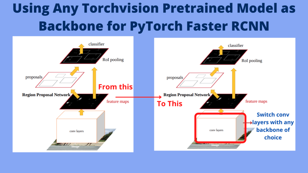
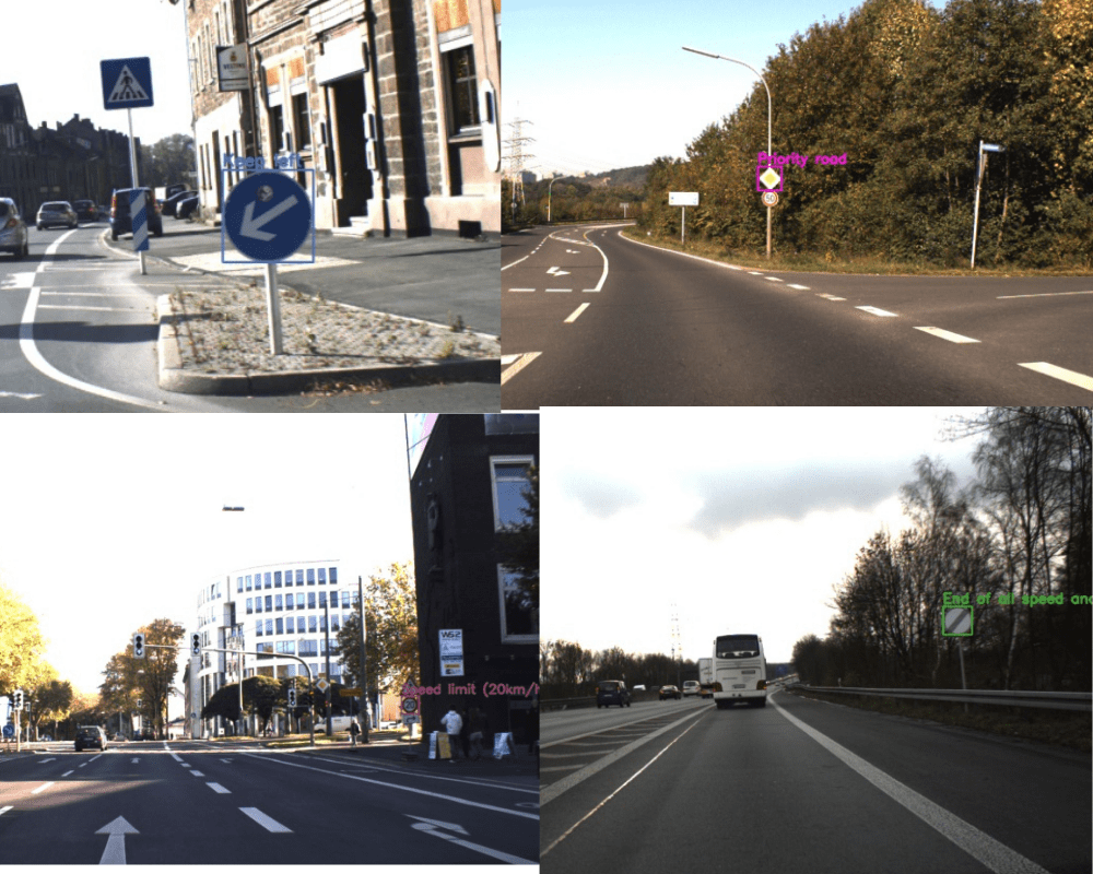
In the last two posts, we covered two things in traffic sign recognition and detection. In the first one, we went through traffic sign recognition using Torchvision pretrained classification models. For that, we used the German Traffic Sign Recognition Benchmark (GTSRB) dataset. And in the previous post, we did traffic sign detection using pretrained PyTorch Faster RCNN models. It was based on the German Traffic Sign Detection Benchmark (GTSDB) dataset. In this post, we will take another approach to prepare the Faster RCNN models to train on the GTSDB dataset. You will get to know how to use any Torchvision pretrained model as backbone for PyTorch Faster RCNN. This will give us the scope to expand our experiments across many Faster RCNN object detection models. And in some cases, even better and faster object detection models.

This is the third post in the traffic sign recognition and detection series.

• Traffic Sign Recognition using PyTorch and Deep Learning.
• Traffic Sign Detection using PyTorch and Pretrained Faster RCNN Model.
• Using Any Torchvision Pretrained Model as Backbone for PyTorch Faster RCNN

But Why This Tutorial?

While many of us may have used PyTorch Faster RCNN object detection models for fine-tuning on their datasets, the choices seem limited. But actually, it is not the case. As I have been experimenting a lot with PyTorch Faster RCNN models recently. I found that we can do a lot more interesting things with the Faster RCNN models. Although a very general and simple approach (yet powerful), as I researched more, I found almost no other resources on the internet covering this. And this idea of creating faster and better object detection models with the Faster RCNN head really excited me. Also, this will help a lot of newcomers in the field who are looking to train custom models on custom datasets.

I am pretty sure that this post will not resurrect the very famous Faster RCNN object detections to the forefront of real-time models. But maybe this will generate a renewed interest in the Faster RCNN models. Maybe someone will take upon the research work on making them better according to today’s real-time standards. Because let’s be honest. With proper training techniques, Faster RCNN models are still able to beat many of today’s models in object detection mAP. It’s just that they are not fast enough to be competitive against models like YOLO, SSD, and other state-of-the-art real-time object detectors.

Topics to Cover in This Tutorial

Before we move into the technical parts of this tutorial, let’s lay out all the points that we will cover here.

• We will start with the discussion for the need of such an approach. The most important question here will be “why do we need to be able to use different pretrained backbones which are not part of the officiail Faster RCNN model?”.
• Then we will move on to a short discussion of the GTSDB dataset, the versions of the frameworks, and the directory structure. These sections will not be very detailed as most of the things remain same as the previous post. Still, we will discuss a few parts where some minor changes take place in the code.
• Next, we will cover the technical part of the tutorial. How to attach any Torchvision pretrained model as backbone to the PyTorch Faster RCNN object detection head? We will go through the code in this section in detail.
• Then we will discuss the training results of three different models on the GTSDB dataset. This is going to be pretty important. As it can make the difference between choosing a model that gives very precision and one that gives high FPS.
• Finally, we will end the tutorial with discussion of a few further steps that we can take to make the project even better.

Why Do We Need to Be Able to Use Any Torchvision Pretrained Model as BackBone for the Faster RCNN Model in PyTorch?

Speaking in general, we have a lot of state-of-the-art real-time object detectors today. Among them, perhaps YOLO models are at the top. They provide good precision along with really high FPS which makes them great for real-time object detection. And almost all of them have one thing in common. They are a one-stage deep learning object detector.

Faster RCNN first came into light in 2015 with the paper – Faster R-CNN: Towards Real-Time Object Detection with Region Proposal Networks. The model was proposed by Shaoqing Ren, Kaiming He, Ross Girshick, and Jian Sun. At the time, it was able to achieve 70.4% mAP on the PASCAL VOC 2012 dataset with a VGG16 backbone which was really high.

Currently, as per Torchvision’s MS COCO pretrained Faster R-CNN ResNet-50 FPN, the mAP is 37.0. This is good but not great. There are other single-stage detectors out there that are a lot faster and have better mAP. The real drawback of Faster RCNN is that it is a two-stage deep learning object detector and therefore. It has a region proposal step which makes it slower compared to other models even with the same mAP.

But there are ways, in which we can make Faster RCNN a lot faster, at least according to today’s standards. One of the best ways is playing around with different backbones and trying to find the right one in terms of FPS and accuracy. For this reason, being able to use any Torchvision pretrained model as a backbone for the PyTorch Faster RCNN model is a nice thing. More details are in the following section.

Current PyTorch Faster RCNN Models and the Approach that We Will Follow

All the posts/tutorials in this traffic recognition/detection series are based on PyTorch 1.10.0 and Torchvision 0.11.1. And as of this version, there are three official Faster RCNN models which are pretrained on the COCO dataset.

• fasterrcnn_resnet50_fpn: Constructs a Faster R-CNN model with a ResNet-50-FPN backbone. It is the slowest of the three available but also capable of giving the highest mAP when fine-tuning on a new dataset.
• fasterrcnn_mobilenet_v3_large_fpn: Constructs a high resolution Faster R-CNN model with a MobileNetV3-Large FPN backbone. Very similar to the Faster RCNN model with the ResNet50 FPN backbone. It is more than twice as fast as the ResNet50 one on the same hardware (GPU). But the mAP takes a considerable hit as a tradeoff because of the high FPS. This was also apparent from the previous tutorial.
• fasterrcnn_mobilenet_v3_large_320_fpn: Constructs a low resolution Faster R-CNN model with a MobileNetV3-Large FPN backbone tuned for mobile use-cases. Almost similar to the above. The only difference is that internally it resizes the images to a minimum size of 320 and maximum size of 640 before feeding to the network. It is slightly faster than the above model. And it is needless to say, for smaller objects, it performs as bad as the MobileNetV3 Large FPN Faster RCNN model or even worse.

From the above points, it is pretty clear that there are two main issues with the available PyTorch pretrained Faster RCNN models. Either they are very fast on a GPU while giving low mAP (MobileNet versions). Or they are slow and give high mAP (ResNet50 version).

What Can We Do to Improve the Situation?

We need to find the right balance between the fastest model possible during inference while getting decent mAP during training. We need to be within considerable mAP range of the Faster RCNN ResNet50 FPN model. That too while not trading away too much speed while inferencing on a GPU (or at least on the same hardware).

Switching backbones is a simple yet very effective strategy to achieve our aim.

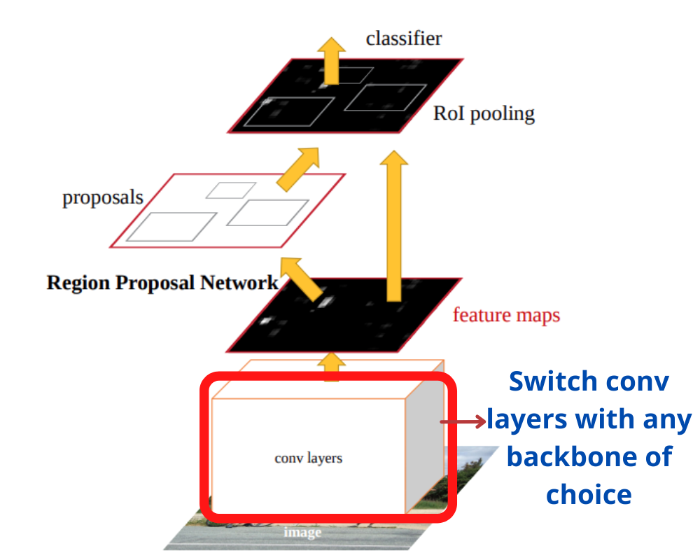
This means that:

• We can use any of the pretrained classification models from Torchvision.
• Then extract their feature layers along with the pretrained weights.
• And use them as backbones with the Faster RCNN head.

Obviously, there are a few other steps we need to complete before we can obtain the final Faster RCNN object detection model. And those steps are mostly for the Faster RCNN architecture. But after obtaining the backbone features, most of the things will be pretty straightforward and almost always the same.

Such an approach of switching backbone can help us train better and more efficient models. Maybe we can still build real-time (or almost real-time) object detection models with Faster RCNN heads. Whatever may be approach and whether or not we are able to build a real-time object detection model with PyTorch. There is going to be a lot of learning, so, it will surely help us build better models in the future.

A few backbones are easy to use and a few are a bit tricky. This is because, for some models, the sequential features are easily available and for some, we have to extract them manually. We will see all these technical details while preparing the model in the coding section.

Download the GTSDB Dataset

If you are starting the series with this post, then you may need to download the GTSDB dataset if you intend to run the code locally.

If you wish to learn more about the dataset, please visit the previous post.

You can visit the link to download them or click on the following direct download links:

• TrainIJCNN2013.zip
• TestIJCNN2013.zip
• gt.txt

There are other data files as well and you will get access to them when downloading the zip file for this tutorial.

Directory Structure

Before moving to the coding section, let’s check out the directory structure of the project.

.
├── inference_outputs
│   ├── images
│   │   ├── 00001.jpg
|   |     ...
│   │   └── 00299.jpg
│   └── videos
│       └── video_1_trimmed_1.mp4
├── input
│   ├── inference_data
│   │   ├── video_1.mp4
│   │   └── video_1_trimmed_1.mp4
│   ├── TestIJCNN2013
│   │   └── TestIJCNN2013Download
│   │       ├── 00000.ppm
│   │       ...
│   │       ├── 00299.ppm
│   │       └── ReadMe.txt
│   ├── TrainIJCNN2013
│   │   ├── 00
│   │   ├── 01
|   |     ...
│   │   ├── 42
│   │   │   
│   │   ├── 00000.ppm
│   │   ...
│   │   ├── 00599.ppm
│   │   ├── ex.txt
│   │   ├── gt.txt
│   │   └── ReadMe.txt
│   ├── train_images
│   │   ├── 00000.ppm
│   │   ...
│   │   └── 00458.ppm
│   ├── train_xmls
│   │   ├── 00000.xml
│   │   ...
│   │   └── 00458.xml
│   ├── valid_images
│   │   ├── 00459.ppm
│   │   ...
│   │   └── 00599.ppm
│   ├── valid_xmls
│   │   ├── 00459.xml
│   │   ...
│   │   └── 00599.xml
│   ├── all_annots.csv
│   ├── classes_list.txt
│   ├── gt.txt
│   ├── MY_README.txt
│   ├── signnames.csv
│   ├── train.csv
│   └── valid.csv
├── outputs
│   ├── last_model.pth
│   └── train_loss.png
├── src
│   ├── models
│   │   ├── fasterrcnn_mobilenetv3_large_320_fpn.py
│   │   ├── fasterrcnn_mobilenetv3_large_fpn.py
│   │   ├── fasterrcnn_resnet18.py
│   │   ├── fasterrcnn_resnet50.py
│   │   ├── fasterrcnn_squeezenet1_0.py
│   │   └── fasterrcnn_squeezenet1_1.py
│   ├── torch_utils
│   │   ├── coco_eval.py
│   │   ├── coco_utils.py
│   │   ├── engine.py
│   │   ├── README.md
│   │   └── utils.py
│   ├── config.py
│   ├── csv_to_xml.py
│   ├── custom_utils.py
│   ├── datasets.py
│   ├── inference.py
│   ├── inference_video.py
│   ├── split_train_valid.py
│   ├── train.py
│   └── txt_to_csv.py

66 directories, 3124 files

In this tutorial, we will not discuss the input, outputs, and inference_outputs directories. They are exactly the same as the previous post. As we are using the same GTSDB dataset, so the images, XML files, and entire structure of the input directory remains the same.

Most of the Python files in the src directory are also the same. If you take a closer look, we have three more Python files in src/models. They are:

• fasterrcnn_resnet18.py
• fasterrcnn_squeezenet1_0.py
• fasterrcnn_squeezenet1_1.py

These are the new Faster RCNN models with ResNet18, SqueezeNet1_0, and SqueezeNet1_1 backbones respectively. And you can already see that the older model files are also present.

Apart from that, there are a few minor changes to the inference scripts which we will also discuss briefly.

As was the case in the previous post, here also, we will not discuss all the Python files. You will still get access to all the Python files while downloading the zip file for this tutorial. But we will mainly discuss the three new model files in detail.

Libraries and Frameworks

As discussed earlier, this entire series uses PyTorch 1.10.0 and Torchvision 0.11.1. Newer versions should also work but older versions may cause issues.

Also, you will need Albumentations for image augmentations.

• Install the latest version of PyTorch from here.
• Install the latest version of Albumentations from here.

Preparing the Dataset

Please follow the Dataset Preprocessing and Creating XML Files section in the previous post to prepare the dataset.

Or you just execute the following three scripts in order to prepare the dataset.

python txt_to_csv.py

python split_train_valid.py

python csv_to_xml.py

Using Any Torchvision Pretrained Model as Backbone for PyTorch Faster RCNN

From here onward, we will discuss the most important code files for this tutorial. And among them, the three new model files which define the PyTorch Faster RCNN object detection models with different backbones come first. All the model preparation code has been inspired by this official PyTorch tutorial. I have tried to make the code more modular so that we can add any model to the codebase and switch with any custom dataset.

We will discuss them in the following order:

• fasterrcnn_squeezenet1_0.py
• fasterrcnn_squeezenet1_1.py
• fasterrcnn_resnet18.py

All three model files are inside the src/models directory. Let’s get into the technical part now.

Faster RCNN Object Detection Model with SqueezeNet1_0 Backbone

The first model that we will discuss uses the SqueezeNet1_0 model features as the backbone. This model was introduced in the paper SqueezeNet: AlexNet-level accuracy with 50x fewer parameters and <0.5MB model size.

The entire SqueezeNet1_0 with 1000 units classification head (for ImageNet classes) has only 1,248,424 parameters. That’s less than 1.25 million parameters. This makes it the first perfect backbone to use for the Faster RCNN object detection model. If you wish the learn more about the pretrained classification model, please check out this tutorial.

There is also another version of it, SqueezeNet1_1 which we will discuss in the next section.

Now, let’s check out the code in fasterrcnn_squeezenet1_0.py and use it as a backbone for the PyTorch Faster RCNN model.

"""
Faster RCNN model with the SqueezeNet1_0 model from Torchvision.
Torchvision link: https://pytorch.org/vision/stable/models.html#id15
Paper: https://arxiv.org/abs/1602.07360
"""

import torchvision

from torchvision.models.detection import FasterRCNN
from torchvision.models.detection.rpn import AnchorGenerator

def create_model(num_classes):
    # Load the pretrained SqueezeNet1_0 backbone.
    backbone = torchvision.models.squeezenet1_0(pretrained=True).features

    # We need the output channels of the last convolutional layers from
    # the features for the Faster RCNN model.
    # It is 512 for SqueezeNet1_0.
    backbone.out_channels = 512

    # Generate anchors using the RPN. Here, we are using 5x3 anchors.
    # Meaning, anchors with 5 different sizes and 3 different aspect 
    # ratios.
    anchor_generator = AnchorGenerator(
        sizes=((32, 64, 128, 256, 512),),
        aspect_ratios=((0.5, 1.0, 2.0),)
    )

    # Feature maps to perform RoI cropping.
    # If backbone returns a Tensor, `featmap_names` is expected to
    # be [0]. We can choose which feature maps to use.
    roi_pooler = torchvision.ops.MultiScaleRoIAlign(
        featmap_names=['0'],
        output_size=7,
        sampling_ratio=2
    )

    # Final Faster RCNN model.
    model = FasterRCNN(
        backbone=backbone,
        num_classes=num_classes,
        rpn_anchor_generator=anchor_generator,
        box_roi_pool=roi_pooler
    )
    print(model)
    return model

The above block contains the entire code we need to create the PyTorch Faster RCNN model with the SqueezeNet1_0 model.

Let’s Go Over the Important Bits of the Above Code

First, we import two classes. They are:

• The FasterRCNN class the we use to build the Faster RCNN model at the end.
• The AnchorGenerator class to generate anchors using the RPN (Region Proposal Network).

Now coming to create_model() function which accepts num_classes (number of classes) as a parameter. On line 14, we load the SqueezeNet1_0 model from torchvision.models. And you can see that we only take the pretrained feature layers from the model. The following is the entire SqueezeNet1_0 model architecture.

SqueezeNet(
  (features): Sequential(
    (0): Conv2d(3, 96, kernel_size=(7, 7), stride=(2, 2))
    (1): ReLU(inplace=True)
    (2): MaxPool2d(kernel_size=3, stride=2, padding=0, dilation=1, ceil_mode=True)
    (3): Fire(
      (squeeze): Conv2d(96, 16, kernel_size=(1, 1), stride=(1, 1))
      (squeeze_activation): ReLU(inplace=True)
      (expand1x1): Conv2d(16, 64, kernel_size=(1, 1), stride=(1, 1))
      (expand1x1_activation): ReLU(inplace=True)
      (expand3x3): Conv2d(16, 64, kernel_size=(3, 3), stride=(1, 1), padding=(1, 1))
      (expand3x3_activation): ReLU(inplace=True)
    )
    (4): Fire(
      (squeeze): Conv2d(128, 16, kernel_size=(1, 1), stride=(1, 1))
      (squeeze_activation): ReLU(inplace=True)
      (expand1x1): Conv2d(16, 64, kernel_size=(1, 1), stride=(1, 1))
      (expand1x1_activation): ReLU(inplace=True)
      (expand3x3): Conv2d(16, 64, kernel_size=(3, 3), stride=(1, 1), padding=(1, 1))
      (expand3x3_activation): ReLU(inplace=True)
    )
    (5): Fire(
      (squeeze): Conv2d(128, 32, kernel_size=(1, 1), stride=(1, 1))
      (squeeze_activation): ReLU(inplace=True)
      (expand1x1): Conv2d(32, 128, kernel_size=(1, 1), stride=(1, 1))
      (expand1x1_activation): ReLU(inplace=True)
      (expand3x3): Conv2d(32, 128, kernel_size=(3, 3), stride=(1, 1), padding=(1, 1))
      (expand3x3_activation): ReLU(inplace=True)
    )
    (6): MaxPool2d(kernel_size=3, stride=2, padding=0, dilation=1, ceil_mode=True)
    (7): Fire(
      (squeeze): Conv2d(256, 32, kernel_size=(1, 1), stride=(1, 1))
      (squeeze_activation): ReLU(inplace=True)
      (expand1x1): Conv2d(32, 128, kernel_size=(1, 1), stride=(1, 1))
      (expand1x1_activation): ReLU(inplace=True)
      (expand3x3): Conv2d(32, 128, kernel_size=(3, 3), stride=(1, 1), padding=(1, 1))
      (expand3x3_activation): ReLU(inplace=True)
    )
    (8): Fire(
      (squeeze): Conv2d(256, 48, kernel_size=(1, 1), stride=(1, 1))
      (squeeze_activation): ReLU(inplace=True)
      (expand1x1): Conv2d(48, 192, kernel_size=(1, 1), stride=(1, 1))
      (expand1x1_activation): ReLU(inplace=True)
      (expand3x3): Conv2d(48, 192, kernel_size=(3, 3), stride=(1, 1), padding=(1, 1))
      (expand3x3_activation): ReLU(inplace=True)
    )
    (9): Fire(
      (squeeze): Conv2d(384, 48, kernel_size=(1, 1), stride=(1, 1))
      (squeeze_activation): ReLU(inplace=True)
      (expand1x1): Conv2d(48, 192, kernel_size=(1, 1), stride=(1, 1))
      (expand1x1_activation): ReLU(inplace=True)
      (expand3x3): Conv2d(48, 192, kernel_size=(3, 3), stride=(1, 1), padding=(1, 1))
      (expand3x3_activation): ReLU(inplace=True)
    )
    (10): Fire(
      (squeeze): Conv2d(384, 64, kernel_size=(1, 1), stride=(1, 1))
      (squeeze_activation): ReLU(inplace=True)
      (expand1x1): Conv2d(64, 256, kernel_size=(1, 1), stride=(1, 1))
      (expand1x1_activation): ReLU(inplace=True)
      (expand3x3): Conv2d(64, 256, kernel_size=(3, 3), stride=(1, 1), padding=(1, 1))
      (expand3x3_activation): ReLU(inplace=True)
    )
    (11): MaxPool2d(kernel_size=3, stride=2, padding=0, dilation=1, ceil_mode=True)
    (12): Fire(
      (squeeze): Conv2d(512, 64, kernel_size=(1, 1), stride=(1, 1))
      (squeeze_activation): ReLU(inplace=True)
      (expand1x1): Conv2d(64, 256, kernel_size=(1, 1), stride=(1, 1))
      (expand1x1_activation): ReLU(inplace=True)
      (expand3x3): Conv2d(64, 256, kernel_size=(3, 3), stride=(1, 1), padding=(1, 1))
      (expand3x3_activation): ReLU(inplace=True)
    )
  )
  (classifier): Sequential(
    (0): Dropout(p=0.5, inplace=False)
    (1): Conv2d(512, 1000, kernel_size=(1, 1), stride=(1, 1))
    (2): ReLU(inplace=True)
    (3): AdaptiveAvgPool2d(output_size=(1, 1))
  )
)

We can see that there total of 12 blocks (highlighted lines) in the Sequential part of the features. These features are used in the backbone defined above. They contain all the pretrained ImageNet weights. After the 12th Fire block the final output channels from the model is 512 which is not quite clear from the above. But we can see that in the classifier that the Conv2d layer has input channels of 512. So, the final output channels value previously was 512. We will see why this is important a bit further on.

Coming back the fasterrcnn_squeezenet1_0.py code again. On line 19, we have defined backbone.out_channels = 512. This is important because we have to mention the exact value of the output channels from the last Conv2d. And it is 512 for the SqueezeNet1_0 model. Now, this backbone is quite ready to be part of the Faster RCNN model.

Next, on line 24, we define the anchor_generator by initializing the AnchorGenerator class. To create the anchor boxes, we choose 5 different anchor sizes with 3 different aspect ratios.

The next step is to define the Region of Interest (RoI) pooler for the feature maps. This we are doing on line 32. We feed the feature maps, the output size for the pooled region, and the sampling ratio for the RoIAlign by initializing the MultiScaleRoIAlign class. Also, it does RoIAling pooling for multiple scales.

The Final Faster RCNN Model

We prepare the final faster RCNN model with the new backbone on line 39. We provide the new backbone, the number of classes (num_classes), the anchor_generator, and the roi_pooler as arguments.

This is the entire process of creating a Faster RCNN model with a new backbone. If you consider everything, then it was not that difficult of a process. Once you have some initial code in place, then you can always change a few things to switch to a new backbone quickly. In most cases, it will the new pretrained features and the final output channels from the 2D convolutional layer.

To make things more concrete, let’s try out two other models.

Faster RCNN Object Detection Model with SqueezeNet1_1 Backbone

The SqueezeNet1_1 is a smaller version of the SqueezeNet1_0 model. It is the next version of the model and is also called SqueenzeNet 1.1. It has 2.4x less computation and slightly fewer parameters than SqueezeNet 1.0. And it does not trade off accuracy for fewer parameters. The number of parameters is just slightly less, that is 1,235,496 parameters. But using it as a backbone should give just a bit of higher speed during inference.

It still, has the same 512 output channels in the final 2D convolutional layer.

Let’s check out the Faster RCNN model code with SqueezeNet1_1 as the backbone and see how easy it is.

This is code for the fasterrcnn_squeezenet1_1.py Python file.

"""
Faster RCNN model with the SqueezeNet1_1 model from Torchvision.
Torchvision link: https://pytorch.org/vision/stable/models.html#id15
SqueezeNet repo: https://github.com/forresti/SqueezeNet/tree/master/SqueezeNet_v1.1
"""

import torchvision

from torchvision.models.detection import FasterRCNN
from torchvision.models.detection.rpn import AnchorGenerator

def create_model(num_classes):
    # Load the pretrained SqueezeNet1_1 backbone.
    backbone = torchvision.models.squeezenet1_1(pretrained=True).features

    # We need the output channels of the last convolutional layers from
    # the features for the Faster RCNN model.
    # It is 512 for SqueezeNet1_1.
    backbone.out_channels = 512

    # Generate anchors using the RPN. Here, we are using 5x3 anchors.
    # Meaning, anchors with 5 different sizes and 3 different aspect 
    # ratios.
    anchor_generator = AnchorGenerator(
        sizes=((32, 64, 128, 256, 512),),
        aspect_ratios=((0.5, 1.0, 2.0),)
    )

    # Feature maps to perform RoI cropping.
    # If backbone returns a Tensor, `featmap_names` is expected to
    # be [0]. We can choose which feature maps to use.
    roi_pooler = torchvision.ops.MultiScaleRoIAlign(
        featmap_names=['0'],
        output_size=7,
        sampling_ratio=2
    )

    # Final Faster RCNN model.
    model = FasterRCNN(
        backbone=backbone,
        num_classes=num_classes,
        rpn_anchor_generator=anchor_generator,
        box_roi_pool=roi_pooler
    )
    print(model)
    return model

As you can see, in this case, we do not change anything except the pretrained model name for the backbone.

Sometimes, changing the backbone can be a bit tricky, especially with models which do not have a features block. We will get to experience that in the next section with the ResNet18 model.

Faster RCNN Object Detection Model with ResNet18 Backbone

ResNet models in the Torchvision library do not have a features block as the SqueezeNet or many other models.

The following is the ResNet18 architecture.

ResNet(
  (conv1): Conv2d(3, 64, kernel_size=(7, 7), stride=(2, 2), padding=(3, 3), bias=False)
  (bn1): BatchNorm2d(64, eps=1e-05, momentum=0.1, affine=True, track_running_stats=True)
  (relu): ReLU(inplace=True)
  (maxpool): MaxPool2d(kernel_size=3, stride=2, padding=1, dilation=1, ceil_mode=False)
  (layer1): Sequential(
    (0): BasicBlock(
      (conv1): Conv2d(64, 64, kernel_size=(3, 3), stride=(1, 1), padding=(1, 1), bias=False)
      (bn1): BatchNorm2d(64, eps=1e-05, momentum=0.1, affine=True, track_running_stats=True)
      (relu): ReLU(inplace=True)
      (conv2): Conv2d(64, 64, kernel_size=(3, 3), stride=(1, 1), padding=(1, 1), bias=False)
      (bn2): BatchNorm2d(64, eps=1e-05, momentum=0.1, affine=True, track_running_stats=True)
    )
    (1): BasicBlock(
      (conv1): Conv2d(64, 64, kernel_size=(3, 3), stride=(1, 1), padding=(1, 1), bias=False)
      (bn1): BatchNorm2d(64, eps=1e-05, momentum=0.1, affine=True, track_running_stats=True)
      (relu): ReLU(inplace=True)
      (conv2): Conv2d(64, 64, kernel_size=(3, 3), stride=(1, 1), padding=(1, 1), bias=False)
      (bn2): BatchNorm2d(64, eps=1e-05, momentum=0.1, affine=True, track_running_stats=True)
    )
  )
  (layer2): Sequential(
    (0): BasicBlock(
      (conv1): Conv2d(64, 128, kernel_size=(3, 3), stride=(2, 2), padding=(1, 1), bias=False)
      (bn1): BatchNorm2d(128, eps=1e-05, momentum=0.1, affine=True, track_running_stats=True)
      (relu): ReLU(inplace=True)
      (conv2): Conv2d(128, 128, kernel_size=(3, 3), stride=(1, 1), padding=(1, 1), bias=False)
      (bn2): BatchNorm2d(128, eps=1e-05, momentum=0.1, affine=True, track_running_stats=True)
      (downsample): Sequential(
        (0): Conv2d(64, 128, kernel_size=(1, 1), stride=(2, 2), bias=False)
        (1): BatchNorm2d(128, eps=1e-05, momentum=0.1, affine=True, track_running_stats=True)
      )
    )
    (1): BasicBlock(
      (conv1): Conv2d(128, 128, kernel_size=(3, 3), stride=(1, 1), padding=(1, 1), bias=False)
      (bn1): BatchNorm2d(128, eps=1e-05, momentum=0.1, affine=True, track_running_stats=True)
      (relu): ReLU(inplace=True)
      (conv2): Conv2d(128, 128, kernel_size=(3, 3), stride=(1, 1), padding=(1, 1), bias=False)
      (bn2): BatchNorm2d(128, eps=1e-05, momentum=0.1, affine=True, track_running_stats=True)
    )
  )
  (layer3): Sequential(
    (0): BasicBlock(
      (conv1): Conv2d(128, 256, kernel_size=(3, 3), stride=(2, 2), padding=(1, 1), bias=False)
      (bn1): BatchNorm2d(256, eps=1e-05, momentum=0.1, affine=True, track_running_stats=True)
      (relu): ReLU(inplace=True)
      (conv2): Conv2d(256, 256, kernel_size=(3, 3), stride=(1, 1), padding=(1, 1), bias=False)
      (bn2): BatchNorm2d(256, eps=1e-05, momentum=0.1, affine=True, track_running_stats=True)
      (downsample): Sequential(
        (0): Conv2d(128, 256, kernel_size=(1, 1), stride=(2, 2), bias=False)
        (1): BatchNorm2d(256, eps=1e-05, momentum=0.1, affine=True, track_running_stats=True)
      )
    )
    (1): BasicBlock(
      (conv1): Conv2d(256, 256, kernel_size=(3, 3), stride=(1, 1), padding=(1, 1), bias=False)
      (bn1): BatchNorm2d(256, eps=1e-05, momentum=0.1, affine=True, track_running_stats=True)
      (relu): ReLU(inplace=True)
      (conv2): Conv2d(256, 256, kernel_size=(3, 3), stride=(1, 1), padding=(1, 1), bias=False)
      (bn2): BatchNorm2d(256, eps=1e-05, momentum=0.1, affine=True, track_running_stats=True)
    )
  )
  (layer4): Sequential(
    (0): BasicBlock(
      (conv1): Conv2d(256, 512, kernel_size=(3, 3), stride=(2, 2), padding=(1, 1), bias=False)
      (bn1): BatchNorm2d(512, eps=1e-05, momentum=0.1, affine=True, track_running_stats=True)
      (relu): ReLU(inplace=True)
      (conv2): Conv2d(512, 512, kernel_size=(3, 3), stride=(1, 1), padding=(1, 1), bias=False)
      (bn2): BatchNorm2d(512, eps=1e-05, momentum=0.1, affine=True, track_running_stats=True)
      (downsample): Sequential(
        (0): Conv2d(256, 512, kernel_size=(1, 1), stride=(2, 2), bias=False)
        (1): BatchNorm2d(512, eps=1e-05, momentum=0.1, affine=True, track_running_stats=True)
      )
    )
    (1): BasicBlock(
      (conv1): Conv2d(512, 512, kernel_size=(3, 3), stride=(1, 1), padding=(1, 1), bias=False)
      (bn1): BatchNorm2d(512, eps=1e-05, momentum=0.1, affine=True, track_running_stats=True)
      (relu): ReLU(inplace=True)
      (conv2): Conv2d(512, 512, kernel_size=(3, 3), stride=(1, 1), padding=(1, 1), bias=False)
      (bn2): BatchNorm2d(512, eps=1e-05, momentum=0.1, affine=True, track_running_stats=True)
    )
  )
  (avgpool): AdaptiveAvgPool2d(output_size=(1, 1))
  (fc): Linear(in_features=512, out_features=1000, bias=True)
)

ResNet18 (and all of the ResNet models in general) have the following structure:

conv => bn1 => relu => maxpool => layer1 => layer2 => layer3 => layer4 => avgpool => fc.

We have to extract all the features till layer4 manually, create a Sequential block out of it, and treat it as a backbone. And it is pretty clear that the backbone.out_channels value is 512 in this case.

Let’s check out the code for fasterrcnn_resnet18.py to make things clearer.

"""
Faster RCNN model with the ResNet18 backbone from Torchvision.
Torchvision link: https://pytorch.org/vision/stable/models.html#id10
ResNet paper: https://arxiv.org/pdf/1512.03385.pdf
"""

import torchvision
import torch.nn as nn

from torchvision.models.detection import FasterRCNN
from torchvision.models.detection.rpn import AnchorGenerator

def create_model(num_classes):
    # Load the pretrained ResNet18 backbone.
    conv1 = torchvision.models.resnet18(pretrained=True).conv1
    bn1 = torchvision.models.resnet18(pretrained=True).bn1
    resnet18_relu = torchvision.models.resnet18(pretrained=True).relu
    resnet18_max_pool = torchvision.models.resnet18(pretrained=True).maxpool
    layer1 = torchvision.models.resnet18(pretrained=True).layer1
    layer2 = torchvision.models.resnet18(pretrained=True).layer2
    layer3 = torchvision.models.resnet18(pretrained=True).layer3
    layer4 = torchvision.models.resnet18(pretrained=True).layer4

    backbone = nn.Sequential(
        conv1, bn1, resnet18_relu, resnet18_max_pool, 
        layer1, layer2, layer3, layer4
    )

    # We need the output channels of the last convolutional layers from
    # the features for the Faster RCNN model.
    # It is 512 for ResNet18.
    backbone.out_channels = 512

    # Generate anchors using the RPN. Here, we are using 5x3 anchors.
    # Meaning, anchors with 5 different sizes and 3 different aspect 
    # ratios.
    anchor_generator = AnchorGenerator(
        sizes=((32, 64, 128, 256, 512),),
        aspect_ratios=((0.5, 1.0, 2.0),)
    )

    # Feature maps to perform RoI cropping.
    # If backbone returns a Tensor, `featmap_names` is expected to
    # be [0]. We can choose which feature maps to use.
    roi_pooler = torchvision.ops.MultiScaleRoIAlign(
        featmap_names=['0'],
        output_size=7,
        sampling_ratio=2
    )

    # Final Faster RCNN model.
    model = FasterRCNN(
        backbone=backbone,
        num_classes=num_classes,
        rpn_anchor_generator=anchor_generator,
        box_roi_pool=roi_pooler
    )
    print(model)
    return model

The most important things happen from lines 15 to 26 in the create_model function. As you can see, we extract the pretrained weights from all layers till layer4. Then we add them to a Sequential block on line 24 which gives the final backbone.

Going over the code a bit on your own will surely help understand this clearly. But after this, we can create a Faster RCNN model by combining almost any of the pretrained classification model’s features as a backbone.

We complete the model preparation explanation here. Before we move on to the training and inference results, let’s check out a few minor changes made to the inference code.

Minor Changes in the Inference Code

Compared to the previous post, we add one new argument parser for the command-line argument flag to both inference.py and inference_video.py. In the last post, we hardcoded the detection threshold. Here, we will provide that as a command-line argument for better controlling the results.

In any case, you do not need to worry if you are downloading the zip file for this tutorial.

Training and Inference Results

We will discuss the training and inference results of the three models discussed. All the experiments were run on a machine with an i7 10th gen CPU, RTX 3080 10GB GPU, and 32GB RAM.

Let’s discuss the results of each of the models.

All the models have been trained for 200 epochs, with an initial learning rate of 0.0001 using AdamW optimizer. We use CosineAnnealingWarmRestarts scheduler to reduce the learning rate uniformly to zero by 225 epochs. This means that the learning rate will be slightly higher than zero in the last few epochs.

For the inference results, we will not visualize the output images. Rather our main focus will be FPS. As the downloadable zip file contains the three models, you are free to run the inference to visualize the outputs.

For changing the model for training, be sure to import the correct model into train.py. The following shows an example of importing fasterrcnn_resnet18.

from models.fasterrcnn_resnet18 import create_model

Similarly, you will need to import the correct model while carrying our image inference and video inference according to the saved model file in outputs directory. These import statements are in inference.py and inference_video.py respectively.

All the training and inference commands are executed from the terminal/command line within the src directory.

After importing the correct model module you just need to execute the following command.

python train.py

Similarly, for image and video inference, execute the following commands respectively. All the inference has been run with a detection confidence threshold of 0.5.

python inference.py --input ../input/TestIJCNN2013/TestIJCNN2013Download --threshold 0.5

python inference_video.py --input ../input/inference_data/video_1_trimmed_1.mp4	--threshold 0.5

You can change the input image directory or input video file if you wish so.

SqueezeNet1_0 Faster RCNN Training Results

The next block shows the truncated training outputs.

Number of training samples: 425
Number of validation samples: 81

FasterRCNN(
  (transform): GeneralizedRCNNTransform(
      Normalize(mean=[0.485, 0.456, 0.406], std=[0.229, 0.224, 0.225])
      Resize(min_size=(800,), max_size=1333, mode='bilinear')
  )
  (backbone): Sequential(
    ...
  (roi_heads): RoIHeads(
    (box_roi_pool): MultiScaleRoIAlign(featmap_names=['0'], output_size=(7, 7), sampling_ratio=2)
    (box_head): TwoMLPHead(
      (fc6): Linear(in_features=25088, out_features=1024, bias=True)
      (fc7): Linear(in_features=1024, out_features=1024, bias=True)
    )
    (box_predictor): FastRCNNPredictor(
      (cls_score): Linear(in_features=1024, out_features=44, bias=True)
      (bbox_pred): Linear(in_features=1024, out_features=176, bias=True)
    )
  )
)
30,099,943 total parameters.
30,099,943 training parameters.

Epoch     0: adjusting learning rate of group 0 to 1.0000e-04.
Epoch: [0]  [  0/107]  eta: 0:01:22  lr: 0.000001  loss: 4.3423 (4.3423)  loss_classifier: 3.5500 (3.5500)  loss_box_reg: 0.0049 (0.0049)  loss_objectness: 0.7657 (0.7657)  loss_rpn_box_reg: 0.0217 (0.0217)  time: 0.7723  data: 0.1869  max mem: 2454
Epoch: [0]  [100/107]  eta: 0:00:00  lr: 0.000101  loss: 0.1153 (0.2645)  loss_classifier: 0.0659 (0.1587)  loss_box_reg: 0.0262 (0.0209)  loss_objectness: 0.0203 (0.0742)  loss_rpn_box_reg: 0.0066 (0.0107)  time: 0.1008  data: 0.0050  max mem: 2796
Epoch: [0]  [106/107]  eta: 0:00:00  lr: 0.000100  loss: 0.1010 (0.2544)  loss_classifier: 0.0546 (0.1525)  loss_box_reg: 0.0201 (0.0207)  loss_objectness: 0.0167 (0.0708)  loss_rpn_box_reg: 0.0064 (0.0104)  time: 0.0968  data: 0.0049  max mem: 2796
Epoch: [0] Total time: 0:00:11 (0.1071 s / it)
creating index...
index created!
Test:  [ 0/21]  eta: 0:00:04  model_time: 0.0353 (0.0353)  evaluator_time: 0.0015 (0.0015)  time: 0.2152  data: 0.1756  max mem: 2796
Test:  [20/21]  eta: 0:00:00  model_time: 0.0335 (0.0328)  evaluator_time: 0.0016 (0.0015)  time: 0.0400  data: 0.0042  max mem: 2796
Test: Total time: 0:00:01 (0.0502 s / it)
Averaged stats: model_time: 0.0335 (0.0328)  evaluator_time: 0.0016 (0.0015)
Accumulating evaluation results...
DONE (t=0.05s).
IoU metric: bbox
 Average Precision  (AP) @[ IoU=0.50:0.95 | area=   all | maxDets=100 ] = 0.000
 Average Precision  (AP) @[ IoU=0.50      | area=   all | maxDets=100 ] = 0.001
 Average Precision  (AP) @[ IoU=0.75      | area=   all | maxDets=100 ] = 0.000
 Average Precision  (AP) @[ IoU=0.50:0.95 | area= small | maxDets=100 ] = 0.000
 Average Precision  (AP) @[ IoU=0.50:0.95 | area=medium | maxDets=100 ] = 0.007
 Average Precision  (AP) @[ IoU=0.50:0.95 | area= large | maxDets=100 ] = -1.000
 Average Recall     (AR) @[ IoU=0.50:0.95 | area=   all | maxDets=  1 ] = 0.001
 Average Recall     (AR) @[ IoU=0.50:0.95 | area=   all | maxDets= 10 ] = 0.007
 Average Recall     (AR) @[ IoU=0.50:0.95 | area=   all | maxDets=100 ] = 0.007
 Average Recall     (AR) @[ IoU=0.50:0.95 | area= small | maxDets=100 ] = 0.001
 Average Recall     (AR) @[ IoU=0.50:0.95 | area=medium | maxDets=100 ] = 0.067
 Average Recall     (AR) @[ IoU=0.50:0.95 | area= large | maxDets=100 ] = -1.000
SAVING PLOTS COMPLETE...
...
Epoch: [199]  [  0/107]  eta: 0:00:37  lr: 0.000004  loss: 0.0053 (0.0053)  loss_classifier: 0.0016 (0.0016)  loss_box_reg: 0.0031 (0.0031)  loss_objectness: 0.0006 (0.0006)  loss_rpn_box_reg: 0.0000 (0.0000)  time: 0.3525  data: 0.2469  max mem: 2796
Epoch: [199]  [100/107]  eta: 0:00:00  lr: 0.000003  loss: 0.0058 (0.0070)  loss_classifier: 0.0017 (0.0023)  loss_box_reg: 0.0036 (0.0044)  loss_objectness: 0.0000 (0.0002)  loss_rpn_box_reg: 0.0000 (0.0001)  time: 0.1037  data: 0.0052  max mem: 2796
^[	Epoch: [199]  [106/107]  eta: 0:00:00  lr: 0.000003  loss: 0.0056 (0.0069)  loss_classifier: 0.0013 (0.0022)  loss_box_reg: 0.0036 (0.0044)  loss_objectness: 0.0000 (0.0002)  loss_rpn_box_reg: 0.0000 (0.0001)  time: 0.0999  data: 0.0051  max mem: 2796
Epoch: [199] Total time: 0:00:11 (0.1063 s / it)
creating index...
index created!
Test:  [ 0/21]  eta: 0:00:05  model_time: 0.0379 (0.0379)  evaluator_time: 0.0023 (0.0023)  time: 0.2547  data: 0.2107  max mem: 2796
Test:  [20/21]  eta: 0:00:00  model_time: 0.0369 (0.0363)  evaluator_time: 0.0027 (0.0028)  time: 0.0461  data: 0.0051  max mem: 2796
Test: Total time: 0:00:01 (0.0588 s / it)
Averaged stats: model_time: 0.0369 (0.0363)  evaluator_time: 0.0027 (0.0028)
Accumulating evaluation results...
DONE (t=0.07s).
IoU metric: bbox
 Average Precision  (AP) @[ IoU=0.50:0.95 | area=   all | maxDets=100 ] = 0.323
 Average Precision  (AP) @[ IoU=0.50      | area=   all | maxDets=100 ] = 0.455
 Average Precision  (AP) @[ IoU=0.75      | area=   all | maxDets=100 ] = 0.368
 Average Precision  (AP) @[ IoU=0.50:0.95 | area= small | maxDets=100 ] = 0.323
 Average Precision  (AP) @[ IoU=0.50:0.95 | area=medium | maxDets=100 ] = 0.642
 Average Precision  (AP) @[ IoU=0.50:0.95 | area= large | maxDets=100 ] = -1.000
 Average Recall     (AR) @[ IoU=0.50:0.95 | area=   all | maxDets=  1 ] = 0.378
 Average Recall     (AR) @[ IoU=0.50:0.95 | area=   all | maxDets= 10 ] = 0.420
 Average Recall     (AR) @[ IoU=0.50:0.95 | area=   all | maxDets=100 ] = 0.420
 Average Recall     (AR) @[ IoU=0.50:0.95 | area= small | maxDets=100 ] = 0.401
 Average Recall     (AR) @[ IoU=0.50:0.95 | area=medium | maxDets=100 ] = 0.683
 Average Recall     (AR) @[ IoU=0.50:0.95 | area= large | maxDets=100 ] = -1.000
SAVING PLOTS COMPLETE...

This is the first result where we use the SqueezeNet1_0 Torchvision pretrained model as backbone for PyTorch Faster RCNN model. We can see that the number of parameters here is higher than the MobileNetV3 Large FPN backbone model from the last tutorial. This higher number of parameters surely helped the model achieved an mAP of 45.5% for IoU=0.50 and mAP of 32.3% for IoU=0.50:0.95.

The following is the training loss plot per iteration.

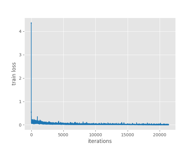
The final training loss here is around 0.0369 which is around 6 times less than the MobileNetV3 Large FPN Faster RCNN model. This result is much better than the MobileNetV3 Large FPN version of Faster RCNN.

SqueezeNet1_0 Faster RCNN Inference Results

Let’s check out the FPS for test image inference and video inference results.

First, the image inference FPS from the Terminal.

TEST PREDICTIONS COMPLETE
Average FPS: 71.200

Now, the video inference FPS.

Average FPS: 74.887

If we consider carefully, these FPS values are just as high as the MobileNetV3 Large FPN version one. While being much higher in mAP and lower in the loss. This is a really good sign.

SqueezeNet1_1 Faster RCNN Training Results

We know that the SqueezeNet1_1 version from Torchvision contains fewer parameters and is less compute-intensive.

Number of training samples: 425
Number of validation samples: 81

FasterRCNN(
  (transform): GeneralizedRCNNTransform(
      Normalize(mean=[0.485, 0.456, 0.406], std=[0.229, 0.224, 0.225])
      Resize(min_size=(800,), max_size=1333, mode='bilinear')
  )
  (backbone): Sequential(
    ...
    (box_predictor): FastRCNNPredictor(
      (cls_score): Linear(in_features=1024, out_features=44, bias=True)
      (bbox_pred): Linear(in_features=1024, out_features=176, bias=True)
    )
  )
)
30,087,015 total parameters.
30,087,015 training parameters.

Epoch     0: adjusting learning rate of group 0 to 1.0000e-04.
Epoch: [0]  [  0/107]  eta: 0:02:15  lr: 0.000001  loss: 4.6265 (4.6265)  loss_classifier: 3.8528 (3.8528)  loss_box_reg: 0.0047 (0.0047)  loss_objectness: 0.7430 (0.7430)  loss_rpn_box_reg: 0.0260 (0.0260)  time: 1.2679  data: 0.6886  max mem: 1692
Epoch: [0]  [100/107]  eta: 0:00:00  lr: 0.000101  loss: 0.1305 (0.2757)  loss_classifier: 0.0783 (0.1722)  loss_box_reg: 0.0274 (0.0224)  loss_objectness: 0.0164 (0.0716)  loss_rpn_box_reg: 0.0057 (0.0095)  time: 0.0884  data: 0.0061  max mem: 2031
Epoch: [0]  [106/107]  eta: 0:00:00  lr: 0.000100  loss: 0.1392 (0.2703)  loss_classifier: 0.0864 (0.1687)  loss_box_reg: 0.0317 (0.0238)  loss_objectness: 0.0165 (0.0685)  loss_rpn_box_reg: 0.0053 (0.0093)  time: 0.0850  data: 0.0058  max mem: 2031
Epoch: [0] Total time: 0:00:10 (0.0951 s / it)
creating index...
index created!
Test:  [ 0/21]  eta: 0:00:04  model_time: 0.0305 (0.0305)  evaluator_time: 0.0016 (0.0016)  time: 0.1995  data: 0.1634  max mem: 2031
Test:  [20/21]  eta: 0:00:00  model_time: 0.0269 (0.0265)  evaluator_time: 0.0012 (0.0012)  time: 0.0336  data: 0.0044  max mem: 2031
Test: Total time: 0:00:00 (0.0432 s / it)
Averaged stats: model_time: 0.0269 (0.0265)  evaluator_time: 0.0012 (0.0012)
Accumulating evaluation results...
DONE (t=0.05s).
IoU metric: bbox
 Average Precision  (AP) @[ IoU=0.50:0.95 | area=   all | maxDets=100 ] = 0.001
 Average Precision  (AP) @[ IoU=0.50      | area=   all | maxDets=100 ] = 0.002
 Average Precision  (AP) @[ IoU=0.75      | area=   all | maxDets=100 ] = 0.000
 Average Precision  (AP) @[ IoU=0.50:0.95 | area= small | maxDets=100 ] = 0.000
 Average Precision  (AP) @[ IoU=0.50:0.95 | area=medium | maxDets=100 ] = 0.033
 Average Precision  (AP) @[ IoU=0.50:0.95 | area= large | maxDets=100 ] = -1.000
 Average Recall     (AR) @[ IoU=0.50:0.95 | area=   all | maxDets=  1 ] = 0.003
 Average Recall     (AR) @[ IoU=0.50:0.95 | area=   all | maxDets= 10 ] = 0.003
 Average Recall     (AR) @[ IoU=0.50:0.95 | area=   all | maxDets=100 ] = 0.003
 Average Recall     (AR) @[ IoU=0.50:0.95 | area= small | maxDets=100 ] = 0.000
 Average Recall     (AR) @[ IoU=0.50:0.95 | area=medium | maxDets=100 ] = 0.033
 Average Recall     (AR) @[ IoU=0.50:0.95 | area= large | maxDets=100 ] = -1.000
SAVING PLOTS COMPLETE...
...
Epoch: [199]  [  0/107]  eta: 0:00:35  lr: 0.000004  loss: 0.0053 (0.0053)  loss_classifier: 0.0018 (0.0018)  loss_box_reg: 0.0034 (0.0034)  loss_objectness: 0.0000 (0.0000)  loss_rpn_box_reg: 0.0000 (0.0000)  time: 0.3285  data: 0.2429  max mem: 2031
Epoch: [199]  [100/107]  eta: 0:00:00  lr: 0.000003  loss: 0.0058 (0.0076)  loss_classifier: 0.0019 (0.0025)  loss_box_reg: 0.0040 (0.0049)  loss_objectness: 0.0000 (0.0001)  loss_rpn_box_reg: 0.0001 (0.0001)  time: 0.0818  data: 0.0051  max mem: 2031
Epoch: [199]  [106/107]  eta: 0:00:00  lr: 0.000003  loss: 0.0058 (0.0079)  loss_classifier: 0.0019 (0.0027)  loss_box_reg: 0.0040 (0.0049)  loss_objectness: 0.0000 (0.0001)  loss_rpn_box_reg: 0.0001 (0.0001)  time: 0.0790  data: 0.0050  max mem: 2031
Epoch: [199] Total time: 0:00:09 (0.0865 s / it)
creating index...
index created!
Test:  [ 0/21]  eta: 0:00:04  model_time: 0.0299 (0.0299)  evaluator_time: 0.0025 (0.0025)  time: 0.2337  data: 0.1977  max mem: 2031
Test:  [20/21]  eta: 0:00:00  model_time: 0.0272 (0.0266)  evaluator_time: 0.0024 (0.0025)  time: 0.0351  data: 0.0045  max mem: 2031
Test: Total time: 0:00:00 (0.0472 s / it)
Averaged stats: model_time: 0.0272 (0.0266)  evaluator_time: 0.0024 (0.0025)
Accumulating evaluation results...
DONE (t=0.07s).
IoU metric: bbox
 Average Precision  (AP) @[ IoU=0.50:0.95 | area=   all | maxDets=100 ] = 0.312
 Average Precision  (AP) @[ IoU=0.50      | area=   all | maxDets=100 ] = 0.427
 Average Precision  (AP) @[ IoU=0.75      | area=   all | maxDets=100 ] = 0.316
 Average Precision  (AP) @[ IoU=0.50:0.95 | area= small | maxDets=100 ] = 0.300
 Average Precision  (AP) @[ IoU=0.50:0.95 | area=medium | maxDets=100 ] = 0.645
 Average Precision  (AP) @[ IoU=0.50:0.95 | area= large | maxDets=100 ] = -1.000
 Average Recall     (AR) @[ IoU=0.50:0.95 | area=   all | maxDets=  1 ] = 0.376
 Average Recall     (AR) @[ IoU=0.50:0.95 | area=   all | maxDets= 10 ] = 0.401
 Average Recall     (AR) @[ IoU=0.50:0.95 | area=   all | maxDets=100 ] = 0.401
 Average Recall     (AR) @[ IoU=0.50:0.95 | area= small | maxDets=100 ] = 0.386
 Average Recall     (AR) @[ IoU=0.50:0.95 | area=medium | maxDets=100 ] = 0.644
 Average Recall     (AR) @[ IoU=0.50:0.95 | area= large | maxDets=100 ] = -1.000
SAVING PLOTS COMPLETE... 

The results are a bit surprising here. The mAP for IoU=0.50:0.95 and IoU=0.50 are surely a bit lower than the SqueezeNet1_0 version. Mostly, we can attribute this to fewer parameters. Interestingly, the loss of 0.0272 is lower than the SqueezeNet1_0 version.

This most probably means that with proper augmentation we can reach just as high as an mAP.

SqueezeNet1_1 Faster RCNN Inference Results

The following are the image inference results.

TEST PREDICTIONS COMPLETE
Average FPS: 87.531

And now, the video inference FPS.

Average FPS: 95.472

This is quite surprising. We are able to reach almost 88 FPS for the images, and 95 FPS for the video inference. The 2.4x less computation is really helping here.

ResNet18 Faster RCNN Training Results

Now, moving on to the Faster RCNN training results with ResNet18 backbone.

Number of training samples: 425
Number of validation samples: 81

FasterRCNN(
  (transform): GeneralizedRCNNTransform(
      Normalize(mean=[0.485, 0.456, 0.406], std=[0.229, 0.224, 0.225])
      Resize(min_size=(800,), max_size=1333, mode='bilinear')
  )
  (backbone): Sequential(
    ...
  (roi_heads): RoIHeads(
    (box_roi_pool): MultiScaleRoIAlign(featmap_names=['0'], output_size=(7, 7), sampling_ratio=2)
    (box_head): TwoMLPHead(
      (fc6): Linear(in_features=25088, out_features=1024, bias=True)
      (fc7): Linear(in_features=1024, out_features=1024, bias=True)
    )
    (box_predictor): FastRCNNPredictor(
      (cls_score): Linear(in_features=1024, out_features=44, bias=True)
      (bbox_pred): Linear(in_features=1024, out_features=176, bias=True)
    )
  )
)
40,541,031 total parameters.
40,541,031 training parameters.

Epoch     0: adjusting learning rate of group 0 to 1.0000e-04.
Epoch: [0]  [  0/107]  eta: 0:01:34  lr: 0.000001  loss: 4.4537 (4.4537)  loss_classifier: 3.7472 (3.7472)  loss_box_reg: 0.0015 (0.0015)  loss_objectness: 0.6966 (0.6966)  loss_rpn_box_reg: 0.0083 (0.0083)  time: 0.8858  data: 0.2344  max mem: 1777
Epoch: [0]  [100/107]  eta: 0:00:00  lr: 0.000101  loss: 0.0641 (0.2183)  loss_classifier: 0.0362 (0.1364)  loss_box_reg: 0.0078 (0.0104)  loss_objectness: 0.0159 (0.0662)  loss_rpn_box_reg: 0.0039 (0.0053)  time: 0.1208  data: 0.0052  max mem: 2243
Epoch: [0]  [106/107]  eta: 0:00:00  lr: 0.000100  loss: 0.0641 (0.2098)  loss_classifier: 0.0362 (0.1309)  loss_box_reg: 0.0089 (0.0104)  loss_objectness: 0.0144 (0.0632)  loss_rpn_box_reg: 0.0037 (0.0053)  time: 0.1159  data: 0.0051  max mem: 2243
Epoch: [0] Total time: 0:00:13 (0.1239 s / it)
creating index...
index created!
Test:  [ 0/21]  eta: 0:00:04  model_time: 0.0445 (0.0445)  evaluator_time: 0.0027 (0.0027)  time: 0.1966  data: 0.1463  max mem: 2243
Test:  [20/21]  eta: 0:00:00  model_time: 0.0366 (0.0357)  evaluator_time: 0.0011 (0.0012)  time: 0.0434  data: 0.0051  max mem: 2243
Test: Total time: 0:00:01 (0.0524 s / it)
Averaged stats: model_time: 0.0366 (0.0357)  evaluator_time: 0.0011 (0.0012)
Accumulating evaluation results...
DONE (t=0.04s).
IoU metric: bbox
 Average Precision  (AP) @[ IoU=0.50:0.95 | area=   all | maxDets=100 ] = 0.000
 Average Precision  (AP) @[ IoU=0.50      | area=   all | maxDets=100 ] = 0.000
 Average Precision  (AP) @[ IoU=0.75      | area=   all | maxDets=100 ] = 0.000
 Average Precision  (AP) @[ IoU=0.50:0.95 | area= small | maxDets=100 ] = 0.000
 Average Precision  (AP) @[ IoU=0.50:0.95 | area=medium | maxDets=100 ] = 0.000
 Average Precision  (AP) @[ IoU=0.50:0.95 | area= large | maxDets=100 ] = -1.000
 Average Recall     (AR) @[ IoU=0.50:0.95 | area=   all | maxDets=  1 ] = 0.000
 Average Recall     (AR) @[ IoU=0.50:0.95 | area=   all | maxDets= 10 ] = 0.000
 Average Recall     (AR) @[ IoU=0.50:0.95 | area=   all | maxDets=100 ] = 0.000
 Average Recall     (AR) @[ IoU=0.50:0.95 | area= small | maxDets=100 ] = 0.000
 Average Recall     (AR) @[ IoU=0.50:0.95 | area=medium | maxDets=100 ] = 0.000
 Average Recall     (AR) @[ IoU=0.50:0.95 | area= large | maxDets=100 ] = -1.000
SAVING PLOTS COMPLETE...
...
Epoch: [199]  [  0/107]  eta: 0:00:39  lr: 0.000004  loss: 0.0078 (0.0078)  loss_classifier: 0.0022 (0.0022)  loss_box_reg: 0.0055 (0.0055)  loss_objectness: 0.0000 (0.0000)  loss_rpn_box_reg: 0.0000 (0.0000)  time: 0.3651  data: 0.2415  max mem: 2243
Epoch: [199]  [100/107]  eta: 0:00:00  lr: 0.000003  loss: 0.0057 (0.0054)  loss_classifier: 0.0019 (0.0017)  loss_box_reg: 0.0033 (0.0037)  loss_objectness: 0.0000 (0.0000)  loss_rpn_box_reg: 0.0000 (0.0000)  time: 0.1175  data: 0.0052  max mem: 2243
Epoch: [199]  [106/107]  eta: 0:00:00  lr: 0.000003  loss: 0.0043 (0.0053)  loss_classifier: 0.0012 (0.0016)  loss_box_reg: 0.0027 (0.0037)  loss_objectness: 0.0000 (0.0000)  loss_rpn_box_reg: 0.0000 (0.0000)  time: 0.1137  data: 0.0051  max mem: 2243
Epoch: [199] Total time: 0:00:12 (0.1206 s / it)
creating index...
index created!
Test:  [ 0/21]  eta: 0:00:05  model_time: 0.0386 (0.0386)  evaluator_time: 0.0020 (0.0020)  time: 0.2684  data: 0.2244  max mem: 2243
Test:  [20/21]  eta: 0:00:00  model_time: 0.0365 (0.0356)  evaluator_time: 0.0025 (0.0025)  time: 0.0443  data: 0.0045  max mem: 2243
Test: Total time: 0:00:01 (0.0576 s / it)
Averaged stats: model_time: 0.0365 (0.0356)  evaluator_time: 0.0025 (0.0025)
Accumulating evaluation results...
DONE (t=0.06s).
IoU metric: bbox
 Average Precision  (AP) @[ IoU=0.50:0.95 | area=   all | maxDets=100 ] = 0.219
 Average Precision  (AP) @[ IoU=0.50      | area=   all | maxDets=100 ] = 0.326
 Average Precision  (AP) @[ IoU=0.75      | area=   all | maxDets=100 ] = 0.230
 Average Precision  (AP) @[ IoU=0.50:0.95 | area= small | maxDets=100 ] = 0.219
 Average Precision  (AP) @[ IoU=0.50:0.95 | area=medium | maxDets=100 ] = 0.317
 Average Precision  (AP) @[ IoU=0.50:0.95 | area= large | maxDets=100 ] = -1.000
 Average Recall     (AR) @[ IoU=0.50:0.95 | area=   all | maxDets=  1 ] = 0.284
 Average Recall     (AR) @[ IoU=0.50:0.95 | area=   all | maxDets= 10 ] = 0.323
 Average Recall     (AR) @[ IoU=0.50:0.95 | area=   all | maxDets=100 ] = 0.323
 Average Recall     (AR) @[ IoU=0.50:0.95 | area= small | maxDets=100 ] = 0.318
 Average Recall     (AR) @[ IoU=0.50:0.95 | area=medium | maxDets=100 ] = 0.356
 Average Recall     (AR) @[ IoU=0.50:0.95 | area= large | maxDets=100 ] = -1.000
SAVING PLOTS COMPLETE...

In spite of being the largest model among the three in terms of parameters, ResNet18 Faster RCNN results are the worst. The final epoch’s mAP at IoU=0.50 is 32.6% and at IoU=0.50:0.95 is 21.9%.

The final epoch’s training loss is 0.0365. As it is a model with a bit different architecture containing residual blocks, maybe training with different hyperameters and learning rate scheduler will help.

ResNet18 Faster RCNN Inference Results

Image inference results.

TEST PREDICTIONS COMPLETE
Average FPS: 72.200

Average FPS: 85.527

For such a large mode, the FPS is quite good. If somehow, we can achieve better mAP, this can be a really good model for real-time predictions.

In conclusion, for now, SqueezeNet1_1 seems to be performing best in terms of speed and accuracy.

Further Steps

For further experiments, you can try creating Faster RCNN models with the following backbones.

• ShuffleNet
• ResNext
• MNASNet

If you find something interesting, you can use the comment section to share your results.

Summary and Conclusion

In this tutorial, we discussed how to use any Torchvision pretrained model as backbone for PyTorch Faster RCNN models. We went through code examples of creating Faster RCNN models with SqueezeNet1_0, SqueezeNet1_1, and ResNet18 models. We also compared the training and inference results. I hope this tutorial was useful to you.

If you have any doubts, thoughts, or suggestions, please leave them in the comment section. I will surely address them.

You can contact me using the Contact section. You can also find me on LinkedIn, and Twitter.