Traffic Sign Recognition using PyTorch and Deep Learning

In this tutorial, we will train a PyTorch deep learning model for traffic sign recognition.

Deep learning and computer vision are advancing many real-life applications today. And some of them are quite revolutionary. The field of autonomous cars/driving is one of them. There is one thing that we need to be quite clear about autonomous driving. It is not just deep learning that is powering the field. Other fields of engineering such as mechanical, electrical, software, and hardware engineering are just as crucial or in some aspects even more so. And deep learning and computer vision happen to be one of them.

And to be fair, we will not be trying to solve any aspect of real-life autonomous driving in this tutorial. Perhaps, not even close. Although we will be training a very simple traffic sign recognition model using PyTorch. That too, using transfer learning and fine-tuning. For this to be successful, we need deep learning and computer vision.

Also, when it comes to traffic signs in autonomous cars, only recognition/classification is not enough. We need to exactly know where the traffic sign is before we can recognize it. Therefore, the detection/localization of traffic signs is a very important part of this. This tutorial will only cover the recognition of traffic signs. In subsequent posts, we will be covering the detection of traffic signs as well.

This is the first post in the traffic sign recognition and detection series.

• Traffic Sign Recognition using PyTorch and Deep Learning.

A Series on Traffic Sign Recognition and Detection

So, starting from this tutorial, it will be a series for traffic sign detection and recognition, interconnected with each other. With this, we will cover a few important aspects and topics for image classification and object detection. These include:

• Traffic Sign Recognition using PyTorch and Deep Learning (this post).
• In the next post we will carry out traffic sign detection using pretrained Faster RCNN models.
• Then we will move on to traffic sign detection using Faster RCNN but with any pretrained backbone from Torchvision.
• Next, we will again go back to traffic sign recognition with custom classification model. We will try to create the smallest yet best performing model possible.
• Finally, traffic sign detection with Faster RCNN with custom backbone pretrained on the traffic sign recognition dataset.

As for the datasets, we will go into the details of the datasets for traffic sign recognition and detection in appropriate sections of the posts. Just for the sake of self-exploration, we will use the following two datasets in the five posts:

• The German Traffic Sign Recognition Benchmark (GTSRB) for traffic sign recognition.
• The German Traffic Sign Detection Benchmark (GTSDB) for traffic sign detection.

With all the details in mind, let’s move on to the next part.

Topics To Cover

We will cover the following points in this tutorial.

• We will start with the exploration of the GTSRB dataset. This will cover:
  • The links to download the datasets.
  • The types of images present along with the number of classes.
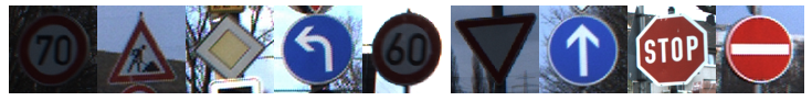
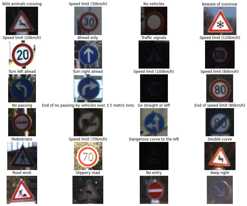
  • Visualizing a few images from the dataset.
• The directory structure for this project/tutorial.
• The coding section for traffic sign recognition using PyTorch and deep learning.
• After training the model, we will also carry out testing along with visualization of class activation maps.

The German Traffic Sign Recognition Benchmark (GTSRB) Dataset

The GTSRB dataset contains images of German road signs across varying classes and scenarios. It is a multi-class dataset with 43 classes and each image is assigned one of the 43 classes.

This dataset was a part of a challenge held at the International Joint Conference on Neural Networks (IJCNN) in 2011. You may also visit the accompanying paper for the dataset here.

• Paper: Man vs. computer: Benchmarking machine learning algorithms for traffic sign recognition.

The entire dataset contains more than 50000 images distributed across 43 classes. Some of the classes are:

• 0 = speed limit 20 (prohibitory)
• 1 = speed limit 30 (prohibitory)
• …
• 10 = no overtaking (trucks) (prohibitory)
• 11 = priority at next intersection (danger)
• …
• 41 = restriction ends (overtaking) (other)
• 42 = restriction ends (overtaking (trucks)) (other)

The files that we are interested in are available via this link. Specifically, we are interested in three files from here. They are GTSRB_Final_Training_Images.zip, GTSRB_Final_Test_Images.zip, and GTSRB_Final_Test_GT.zip.

The GTSRB_Final_Training_Images.zip contains a total of 39209 images in their respective class folders. We will split this into a training and validation set.

The GTSRB_Final_Test_Images.zip contains 12631 images for testing. It does not contain any class folder division. We will use this for testing and GTSRB_Final_Test_GT.zip contains a CSV file with the ground truth classes for all the test images.

GTSRB_Final_Training_Images
└── GTSRB
    ├── Final_Training
    │   └── Images
    │       ├── 00000 [211 entries exceeds filelimit, not opening dir]
    │       ├── 00001 [2221 entries exceeds filelimit, not opening dir]
            ...
    │       ├── 00039 [301 entries exceeds filelimit, not opening dir]
    │       ├── 00040 [361 entries exceeds filelimit, not opening dir]
    │       ├── 00041 [241 entries exceeds filelimit, not opening dir]
    │       └── 00042 [241 entries exceeds filelimit, not opening dir]
    └── Readme-Images.txt
GTSRB_Final_Test_Images
└── GTSRB
    ├── Final_Test
    │   └── Images [12631 entries exceeds filelimit, not opening dir]
    └── Readme-Images-Final-test.txt
GTSRB_Final_Test_GT
└── GT-final_test.csv

As you can see, the GTSRB_Final_Training_Images/GTSRB/Final_Training/Images contains the class folders with numbers according to the classes. But we also need the class names for the final testing of the trained model. There is another CSV file mapping all the class numbers to the traffic sign names. It is the signnames.csv file that you will get access to while downloading the zip file for this tutorial.

Download the Files

You can either download the files on your own from this webpage. Or you can click on the following to access the direct download links for the files that we need.

• GTSRB_Final_Training_Images.zip
• GTSRB_Final_Test_Images.zip
• GTSRB_Final_Test_GT.zip

For now, you can download these and we will discuss the directory structure in the next section.

Directory Structure

The following is the directory structure for the project.

├── input
│   ├── GTSRB_Final_Test_GT
│   │   └── GT-final_test.csv
│   ├── GTSRB_Final_Test_Images
│   │   └── GTSRB
│   │       ├── Final_Test
│   │       │   └── Images [12631 entries exceeds filelimit, not opening dir]
│   │       └── Readme-Images-Final-test.txt
│   ├── GTSRB_Final_Training_Images
│   │   └── GTSRB
│   │       ├── Final_Training
│   │       │   └── Images
│   │       │       ├── 00000 [211 entries exceeds filelimit, not opening dir]
│   │       │       ├── 00001 [2221 entries exceeds filelimit, not opening dir]
                    ...
│   │       │       ├── 00040 [361 entries exceeds filelimit, not opening dir]
│   │       │       ├── 00041 [241 entries exceeds filelimit, not opening dir]
│   │       │       └── 00042 [241 entries exceeds filelimit, not opening dir]
│   │       └── Readme-Images.txt
│   ├── README.txt
│   └── signnames.csv
├── outputs
│   ├── test_results [12630 entries exceeds filelimit, not opening dir]
│   ├── accuracy.png
│   ├── loss.png
│   └── model.pth
└── src
    ├── cam.py
    ├── datasets.py
    ├── model.py
    ├── train.py
    └── utils.py

• The input directory has all the datasets that we need. This also contains the signnames.csv which we need to map the class number to class labels while doing the final testing of the model.
• The outputs directory contains the results from training and testing. These include the plots, the trained model, and the resulting test images.
• And the src directory contains the Python code files.

Be sure to download the zip file and extract it. It contains the Python code files along with the signnames.csv file in the input directory and also all the outputs along with the trained model.

Libraries and Frameworks to Install

For the libraries and frameworks, there are two important ones. They are PyTorch and Albumentations. All code for this tutorial has been developed with PyTorch 1.10.0 and Albumentations 1.1.0.

Mostly, you can also go with whatever latest versions of the libraries are available at the time of your reading this. If you face issues, then the mentioned versions will surely work smoothly.

• Install the latest version of PyTorch from here.
• Install the latest version of Albumentations from here.

Traffic Sign Recognition using PyTorch and Deep Learning

The above sections cover all the setup steps for traffic sign recognition using PyTorch and deep learning. Now, we can get on with the coding part of the tutorial.

As we can see, there are five Python files for this tutorial. Before we can start the training, we need the code for utils.py, datasets.py, model.py, and train.py. After we have the trained model with us, we will use the cam.py script for testing the model and visualizing the class activation maps.

All the code files will be present in the src directory. We will start the helper functions and training utilities as usual.

Helper Functions

The helper functions will go into the utils.py file. And as in many of the previous image classification posts, this contains two functions. One for saving the trained model, and for saving the loss and accuracy graphs to disk.

The following code block contains the imports and the save_model() function.

import torch
import matplotlib
import matplotlib.pyplot as plt

matplotlib.style.use('ggplot')

def save_model(epochs, model, optimizer, criterion):
    """
    Function to save the trained model to disk.
    """
    torch.save({
                'epoch': epochs,
                'model_state_dict': model.state_dict(),
                'optimizer_state_dict': optimizer.state_dict(),
                'loss': criterion,
                }, f"../outputs/model.pth")

Along with the model state dictionary, we are also saving the number of epochs, the optimizer state dictionary, and also, the loss functions. With this, we can easily resume training whenever needed.

The next code block is for saving the loss and accuracy graphs.

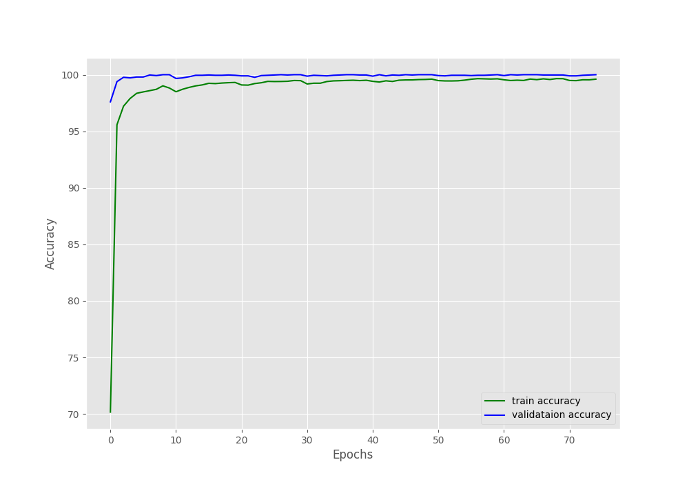
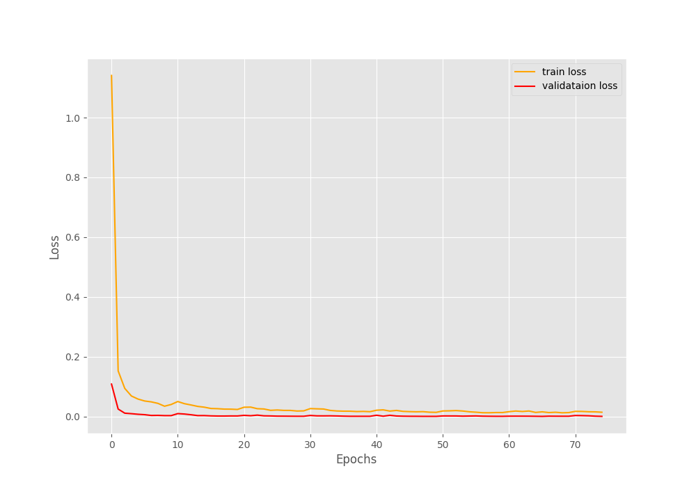
def save_plots(train_acc, valid_acc, train_loss, valid_loss):
    """
    Function to save the loss and accuracy plots to disk.
    """
    # Accuracy plots.
    plt.figure(figsize=(10, 7))
    plt.plot(
        train_acc, color='green', linestyle='-', 
        label='train accuracy'
    )
    plt.plot(
        valid_acc, color='blue', linestyle='-', 
        label='validataion accuracy'
    )
    plt.xlabel('Epochs')
    plt.ylabel('Accuracy')
    plt.legend()
    plt.savefig(f"../outputs/accuracy.png")
    
    # Loss plots.
    plt.figure(figsize=(10, 7))
    plt.plot(
        train_loss, color='orange', linestyle='-', 
        label='train loss'
    )
    plt.plot(
        valid_loss, color='red', linestyle='-', 
        label='validataion loss'
    )
    plt.xlabel('Epochs')
    plt.ylabel('Loss')
    plt.legend()
    plt.savefig(f"../outputs/loss.png") 

The function accepts lists containing the respective accuracy and loss values and saves the plots to disk.

Preparing the Dataset

The dataset preparation part is going to be a bit important here. Although there are enough images (around 40000) for training and validation, still, we will use augmentations.

Now, remember that these are traffic sign images. We cannot use the most common ones like horizontal and vertical flipping. That may change the meaning of the sign entirely. Instead, we will use Albumentations to try and simulate some real-world augmentations. We will take a look at those when writing the code.

The code for dataset preparation will go into the datasets.py file.

First, the import statements, and defining the constants.

import torch
import albumentations as A
import numpy as np

from torchvision import datasets
from torch.utils.data import DataLoader, Subset
from albumentations.pytorch import ToTensorV2

# Required constants.
ROOT_DIR = '../input/GTSRB_Final_Training_Images/GTSRB/Final_Training/Images'
VALID_SPLIT = 0.1
RESIZE_TO = 224 # Image size of resize when applying transforms.
BATCH_SIZE = 128
NUM_WORKERS = 4 # Number of parallel processes for data preparation.

For the constants, we define the:

• Data folder path.
• The validation split, that is 10%.
• Size for image resizing.
• The batch size.
• And number of workers for parallel processing.

The Training and Validation Transforms and Augmentations

Now, coming to the important part. The transforms and augmentations. Let’s take a look at the code first.

# Training transforms.
class TrainTransforms:
    def __init__(self, resize_to):
        self.transforms = A.Compose([
            A.Resize(resize_to, resize_to),
            A.RandomBrightnessContrast(),
            A.RandomFog(),
            A.RandomRain(),
            A.Normalize(
                mean=[0.485, 0.456, 0.406],
                std=[0.229, 0.224, 0.225]
                ),
            ToTensorV2()
        ])
    
    def __call__(self, img):
        return self.transforms(image=np.array(img))['image']

# Validation transforms.
class ValidTransforms:
    def __init__(self, resize_to):
        self.transforms = A.Compose([
            A.Resize(resize_to, resize_to),
            A.Normalize(
                mean=[0.485, 0.456, 0.406],
                std=[0.229, 0.224, 0.225]
                ),
            ToTensorV2()
        ])
    
    def __call__(self, img):
        return self.transforms(image=np.array(img))['image']

We define two classes, TrainTransforms and ValidTransforms for training and validation data respectively.

In the TrainTransforms:

• We define the transforms variable in the __init__() method.
• First, we resize the image to the desired size.
• Then, we apply the RandomBrightnessContrast, RandomFog, and RandomRain augmentations from Albumentations.
• Finally, we apply the processing transforms such as normalizing the values using ImageNet mean and standard deviation and converting the images to tensors. The ImageNet stats are needed as we will use a pretrained model.
• Whenever we initialize TrainTransforms, the __call__() method will be executed passing the image through self.transforms.

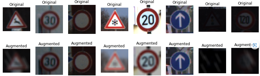
Note that we use the default values of the augmentations with a probability of 0.5 (also default).

Although not entirely, the above augmentations should be able to simulate real-world cases to some extent. In case, you are wondering how the images look after passing through the augmentations, the following figure shows just that.

Coming to the validation transform now. Generally, we do not apply any augmentations to the validation images, so, we just apply the preprocessing transforms.

Datasets and DataLoaders for Training and Validation

Now, we will write two more functions. One for preparing the training and validation dataset, and another for the data loaders.

def get_datasets():
    """
    Function to prepare the Datasets.

    Returns the training and validation datasets along 
    with the class names.
    """
    dataset = datasets.ImageFolder(
        ROOT_DIR, 
        transform=(TrainTransforms(RESIZE_TO))
    )
    dataset_test = datasets.ImageFolder(
        ROOT_DIR, 
        transform=(ValidTransforms(RESIZE_TO))
    )
    dataset_size = len(dataset)

    # Calculate the validation dataset size.
    valid_size = int(VALID_SPLIT*dataset_size)
    # Radomize the data indices.
    indices = torch.randperm(len(dataset)).tolist()
    # Training and validation sets.
    dataset_train = Subset(dataset, indices[:-valid_size])
    dataset_valid = Subset(dataset_test, indices[-valid_size:])

    return dataset_train, dataset_valid, dataset.classes

def get_data_loaders(dataset_train, dataset_valid):
    """
    Prepares the training and validation data loaders.

    :param dataset_train: The training dataset.
    :param dataset_valid: The validation dataset.

    Returns the training and validation data loaders.
    """
    train_loader = DataLoader(
        dataset_train, batch_size=BATCH_SIZE, 
        shuffle=True, num_workers=NUM_WORKERS
    )
    valid_loader = DataLoader(
        dataset_valid, batch_size=BATCH_SIZE, 
        shuffle=False, num_workers=NUM_WORKERS
    )
    return train_loader, valid_loader

The above two functions are pretty much self-explanatory. Only a few things to note here. We use the ImageFolder class for preparing the training and validation datasets. Also, we pass the TrainTransforms and ValidTransforms to the transform argument at the respective places (lines 56 and 60).

The get_data_loaders() function returns the train_loader and valid_loader.

The Neural Network Model

We will use the pretrained MobileNetV3 Large model for traffic sign recognition using PyTorch and deep learning. The main reason for using this is the small number of parameters (just above 4 million) and how well it works when used with proper augmentations.

The neural network model code will go into the model.py file.

import torchvision.models as models
import torch.nn as nn

def build_model(pretrained=True, fine_tune=False, num_classes=10):
    if pretrained:
        print('[INFO]: Loading pre-trained weights')
    else:
        print('[INFO]: Not loading pre-trained weights')
    model = models.mobilenet_v3_large(pretrained=pretrained)

    if fine_tune:
        print('[INFO]: Fine-tuning all layers...')
        for params in model.parameters():
            params.requires_grad = True
    elif not fine_tune:
        print('[INFO]: Freezing hidden layers...')
        for params in model.parameters():
            params.requires_grad = False

    # Change the final classification head.
    model.classifier[3] = nn.Linear(in_features=1280, out_features=num_classes)
    return model

The above function will return the model instance based on whether we want to load the pretrained weights or not and also want to fine-tune all the layers or not.

The Training Script

In this section, we will cover the training script code. This will be long but simple. In short, we will connect all the components from the previous modules.

We will write the training script code in train.py.

First, we will import all the required modules and libraries, set the seed for reproducibility, and construct the argument parser.

import torch
import argparse
import torch.nn as nn
import torch.optim as optim
import time

from tqdm.auto import tqdm

from model import build_model
from datasets import get_datasets, get_data_loaders
from utils import save_model, save_plots

seed = 42
torch.manual_seed(seed)
torch.cuda.manual_seed(seed)
torch.backends.cudnn.deterministic = True
torch.backends.cudnn.benchmark = True

# Construct the argument parser.
parser = argparse.ArgumentParser()
parser.add_argument(
    '-e', '--epochs', type=int, default=10,
    help='Number of epochs to train our network for'
)
parser.add_argument(
    '-lr', '--learning-rate', type=float,
    dest='learning_rate', default=0.001,
    help='Learning rate for training the model'
)
parser.add_argument(
    '-pw', '--pretrained', action='store_true', 
    help='whether to use pretrained weihgts or not'
)
parser.add_argument(
    '-ft', '--fine-tune', dest='fine_tune', action='store_true',
    help='whether to train all layers or not'
)
args = vars(parser.parse_args())

Setting the seed will ensure that we will get the same results with each run.

For the argument parser, we have the following flags:

• --epochs: For specifying the number of epochs to train for.
• --learning-rate: To control the learning rate. We can control it from the command line directly. When using pretrained weights, a lower learning rate works better.
• --pretrained: To specify whether to use pretrained weights or not.
• --fine-tune: Whether we want to train all hidden layers or not.

The Training Function

The following code block defines the training function.

# Training function.
def train(
    model, trainloader, optimizer, 
    criterion, scheduler=None, epoch=None
):
    model.train()
    print('Training')
    train_running_loss = 0.0
    train_running_correct = 0
    counter = 0
    iters = len(trainloader)
    for i, data in tqdm(enumerate(trainloader), total=len(trainloader)):
        counter += 1
        image, labels = data
        image = image.to(device)
        labels = labels.to(device)
        optimizer.zero_grad()
        # Forward pass.
        outputs = model(image)
        # Calculate the loss.
        loss = criterion(outputs, labels)
        train_running_loss += loss.item()
        # Calculate the accuracy.
        _, preds = torch.max(outputs.data, 1)
        train_running_correct += (preds == labels).sum().item()
        # Backpropagation.
        loss.backward()
        # Update the weights.
        optimizer.step()

        if scheduler is not None:
            scheduler.step(epoch + i / iters)
    
    # Loss and accuracy for the complete epoch.
    epoch_loss = train_running_loss / counter
    epoch_acc = 100. * (train_running_correct / len(trainloader.dataset))
    return epoch_loss, epoch_acc

It is a very simple and general training function for image classification in PyTorch. One important thing is the scheduler parameter. We can pass the CosineAnnealingWarmRestarts scheduler when calling the function which will execute line 69.

With the learning rate scheduler, the final training accuracy is about 0.5% higher. This may not seem much, but let’s squeeze out whatever performance we can out of our neural network model.

If you wish to learn more about the Cosine Annealing with Warm Restarts scheduler, you can visit this post which covers a more detailed view of the concept.

The Validation Function

# Validation function.
def validate(model, testloader, criterion, class_names):
    model.eval()
    print('Validation')
    valid_running_loss = 0.0
    valid_running_correct = 0
    counter = 0

    # We need two lists to keep track of class-wise accuracy.
    class_correct = list(0. for i in range(len(class_names)))
    class_total = list(0. for i in range(len(class_names)))

    with torch.no_grad():
        for i, data in tqdm(enumerate(testloader), total=len(testloader)):
            counter += 1
            
            image, labels = data
            image = image.to(device)
            labels = labels.to(device)
            # Forward pass.
            outputs = model(image)
            # Calculate the loss.
            loss = criterion(outputs, labels)
            valid_running_loss += loss.item()
            # Calculate the accuracy.
            _, preds = torch.max(outputs.data, 1)
            valid_running_correct += (preds == labels).sum().item()

            # Calculate the accuracy for each class.
            correct  = (preds == labels).squeeze()
            for i in range(len(preds)):
                label = labels[i]
                class_correct[label] += correct[i].item()
                class_total[label] += 1
        
    # Loss and accuracy for the complete epoch.
    epoch_loss = valid_running_loss / counter
    epoch_acc = 100. * (valid_running_correct / len(testloader.dataset))

    # Print the accuracy for each class after every epoch.
    print('\n')
    for i in range(len(class_names)):
        print(f"Accuracy of class {class_names[i]}: {100*class_correct[i]/class_total[i]}")
    print('\n')
    return epoch_loss, epoch_acc

We don’t need the backpropagation here. But we are calculating the per-class accuracy here which will be useful to note which classes are particularly difficult to learn. We calculate that starting from lines 105 to 109. And we print those accuracies on line 118.

The Main Code Block

The main code block (if __name__ == '__main__') will just define every variable, call every function, and start the training loop.

if __name__ == '__main__':
    # Load the training and validation datasets.
    dataset_train, dataset_valid, dataset_classes = get_datasets()
    print(f"[INFO]: Number of training images: {len(dataset_train)}")
    print(f"[INFO]: Number of validation images: {len(dataset_valid)}")
    print(f"[INFO]: Class names: {dataset_classes}\n")
    # Load the training and validation data loaders.
    train_loader, valid_loader = get_data_loaders(dataset_train, dataset_valid)

    # Learning_parameters. 
    lr = args['learning_rate']
    epochs = args['epochs']
    device = ('cuda' if torch.cuda.is_available() else 'cpu')
    print(f"Computation device: {device}")
    print(f"Learning rate: {lr}")
    print(f"Epochs to train for: {epochs}\n")

    # Load the model.
    model = build_model(
        pretrained=args['pretrained'],
        fine_tune=args['fine_tune'], 
        num_classes=len(dataset_classes)
    ).to(device)
    
    # Total parameters and trainable parameters.
    total_params = sum(p.numel() for p in model.parameters())
    print(f"{total_params:,} total parameters.")
    total_trainable_params = sum(
        p.numel() for p in model.parameters() if p.requires_grad)
    print(f"{total_trainable_params:,} training parameters.")

    # Optimizer.
    optimizer = optim.Adam(model.parameters(), lr=lr)
    # Loss function.
    criterion = nn.CrossEntropyLoss()

    scheduler = torch.optim.lr_scheduler.CosineAnnealingWarmRestarts(
        optimizer, 
        T_0=10, 
        T_mult=1,
        verbose=True
    )

    # Lists to keep track of losses and accuracies.
    train_loss, valid_loss = [], []
    train_acc, valid_acc = [], []
    # Start the training.
    for epoch in range(epochs):
        print(f"[INFO]: Epoch {epoch+1} of {epochs}")
        train_epoch_loss, train_epoch_acc = train(
            model, train_loader, 
            optimizer, criterion,
            scheduler=scheduler, epoch=epoch
        )
        valid_epoch_loss, valid_epoch_acc = validate(model, valid_loader,  
                                                    criterion, dataset_classes)
        train_loss.append(train_epoch_loss)
        valid_loss.append(valid_epoch_loss)
        train_acc.append(train_epoch_acc)
        valid_acc.append(valid_epoch_acc)
        print(f"Training loss: {train_epoch_loss:.3f}, training acc: {train_epoch_acc:.3f}")
        print(f"Validation loss: {valid_epoch_loss:.3f}, validation acc: {valid_epoch_acc:.3f}")
        print('-'*50)
        time.sleep(5)
        
    # Save the trained model weights.
    save_model(epochs, model, optimizer, criterion)
    # Save the loss and accuracy plots.
    save_plots(train_acc, valid_acc, train_loss, valid_loss)
    print('TRAINING COMPLETE')

The following things happen in the above code block:

• We start with preparing the datasets and data loaders (lines 123 and 128).
• From line 131, we define the learning parameters like learning rate, epochs, and the computation device also.
• Then we build the model, define the optimizer and the loss function.
• Line 157 defines the CosineAnnealingWarmRestarts scheduler which will restart the learning rate every 10 epochs.
• The training loop starts from line 168. After the training completes, we save the model and the accuracy and loss plots.

This completes the coding part that we need for training our model. In the next section, we will check the training results.

Executing train.py

Within the src directory, execute the following command in your terminal/command line.

python train.py --pretrained --fine-tune --epochs 75 --learning-rate 0.0001

We are using the pretrained weights, fine-tuning all layers, and training for 75 epochs with an initial learning rate of 0.0001.

Let’s check out the terminal outputs.

[INFO]: Number of training images: 35289
[INFO]: Number of validation images: 3920
[INFO]: Class names: ['00000', '00001', '00002', '00003', '00004', '00005', '00006', '00007', '00008', '00009', '00010', '00011', '00012', '00013', '00014', '00015', '00016', '00017', '00018', '00019', '00020', '00021', '00022', '00023', '00024', '00025', '00026', '00027', '00028', '00029', '00030', '00031', '00032', '00033', '00034', '00035', '00036', '00037', '00038', '00039', '00040', '00041', '00042']

Computation device: cuda
Learning rate: 0.0001
Epochs to train for: 75

[INFO]: Loading pre-trained weights
[INFO]: Fine-tuning all layers...
4,257,115 total parameters.
4,257,115 training parameters.
Epoch     0: adjusting learning rate of group 0 to 1.0000e-04.
[INFO]: Epoch 1 of 75
Training
100%|████████████████████████████████████████████████████████████████████████████████████████████████████████████████████████████████████████████████████████████████████████████| 276/276 [00:45<00:00,  6.05it/s]
Validation
100%|██████████████████████████████████████████████████████████████████████████████████████████████████████████████████████████████████████████████████████████████████████████████| 31/31 [00:02<00:00, 15.27it/s]


Accuracy of class 00000: 96.0
Accuracy of class 00001: 99.17695473251028
Accuracy of class 00002: 96.88888888888889
...
Accuracy of class 00040: 96.66666666666667
Accuracy of class 00041: 75.0
Accuracy of class 00042: 95.65217391304348


Training loss: 1.141, training acc: 70.164
Validation loss: 0.108, validation acc: 97.602
...
[INFO]: Epoch 75 of 75
Training
100%|████████████████████████████████████████████████████████████████████████████████████████████████████████████████████████████████████████████████████████████████████████████| 276/276 [00:38<00:00,  7.14it/s]
Validation
100%|██████████████████████████████████████████████████████████████████████████████████████████████████████████████████████████████████████████████████████████████████████████████| 31/31 [00:01<00:00, 18.58it/s]


Accuracy of class 00000: 100.0
Accuracy of class 00001: 100.0
Accuracy of class 00002: 100.0
...
Accuracy of class 00040: 100.0
Accuracy of class 00041: 100.0
Accuracy of class 00042: 100.0


Training loss: 0.014, training acc: 99.606
Validation loss: 0.000, validation acc: 100.000
--------------------------------------------------
TRAINING COMPLETE

After 75 epochs, the validation loss is 0, validation accuracy is 100%, training loss is 0.014, and training accuracy is 99.6%. Because we applied augmentations to the training set, it is relatively difficult to learn. Maybe using a slightly less intense augmentation method will give us 100% training accuracy also. But for now, we will go with these results.

The following are the accuracy and loss graphs.

We are done with the training part as of now and have the saved model also. In the next section, we will cover the test script which will also give us visualizations for class activation maps.

Testing the Model and Visualizing Class Activation Maps

We will test the trained model on the images present in the input/GTSRB_Final_Test_Images/GTSRB/Final_Test/Images directory. The ground truth for these images is present in the input/GTSRB_Final_Test_GT/GT-final_test.csv file.

The code for this will go into the cam.py file.

We will not go through a detailed explanation of the test script here. Instead, we will just put the code inside their subsections with a brief heading.

But you can find all the details about class activation maps in the following:

• Basic Introduction to Class Activation Maps in Deep Learning using PyTorch
• PyTorch Class Activation Map using Custom Trained Model

Here, you will find the original CAM code which I modified a bit in this script.

And the rest of the script is just simple inference on images using our trained model.

Imports, Set Up, and Loading the Model

import numpy as np
import cv2
import torch
import glob as glob
import pandas as pd
import os
import albumentations as A
import time

from albumentations.pytorch import ToTensorV2
from torch.nn import functional as F
from torch import topk

from model import build_model

# Define computation device.
device = 'cpu'
# Class names.
sign_names_df = pd.read_csv('../input/signnames.csv')
class_names = sign_names_df.SignName.tolist()

# DataFrame for ground truth.
gt_df = pd.read_csv(
    '../input/GTSRB_Final_Test_GT/GT-final_test.csv', 
    delimiter=';'
)
gt_df = gt_df.set_index('Filename', drop=True)

# Initialize model, switch to eval model, load trained weights.
model = build_model(
    pretrained=False,
    fine_tune=False, 
    num_classes=43
).to(device)
model = model.eval()
model.load_state_dict(
    torch.load(
        '../outputs/model.pth', map_location=device
    )['model_state_dict']
)

Apply Class Activation Map Results, Apply the Class Activation Map Colors on Original Image, and Function to Return the Final CAM Image

# https://github.com/zhoubolei/CAM/blob/master/pytorch_CAM.py
def returnCAM(feature_conv, weight_softmax, class_idx):
    # Generate the class activation maps upsample to 256x256.
    size_upsample = (256, 256)
    bz, nc, h, w = feature_conv.shape
    output_cam = []
    for idx in class_idx:
        cam = weight_softmax[idx].dot(feature_conv.reshape((nc, h*w)))
        cam = cam.reshape(h, w)
        cam = cam - np.min(cam)
        cam_img = cam / np.max(cam)
        cam_img = np.uint8(255 * cam_img)
        output_cam.append(cv2.resize(cam_img, size_upsample))
    return output_cam

def apply_color_map(CAMs, width, height, orig_image):
    for i, cam in enumerate(CAMs):
        heatmap = cv2.applyColorMap(cv2.resize(cam,(width, height)), cv2.COLORMAP_JET)
        result = heatmap * 0.5 + orig_image * 0.5
        result = cv2.resize(result, (224, 224))
        return result

def visualize_and_save_map(
    result, orig_image, gt_idx=None, class_idx=None, save_name=None
):
    # Put class label text on the result.
    if class_idx is not None:
        cv2.putText(
            result, 
            f"Pred: {str(class_names[int(class_idx)])}", (5, 20), 
            cv2.FONT_HERSHEY_SIMPLEX, 0.55, (0, 255, 0), 2,
            cv2.LINE_AA
        )
    if gt_idx is not None:
        cv2.putText(
            result, 
            f"GT: {str(class_names[int(gt_idx)])}", (5, 40), 
            cv2.FONT_HERSHEY_SIMPLEX, 0.55, (0, 255, 0), 2,
            cv2.LINE_AA
        )
    # cv2.imshow('CAM', result/255.)
    orig_image = cv2.resize(orig_image, (224, 224))
    # cv2.imshow('Original image', orig_image)
    img_concat = cv2.hconcat([
        np.array(result, dtype=np.uint8), 
        np.array(orig_image, dtype=np.uint8)
    ])
    cv2.imshow('Result', img_concat)
    cv2.waitKey(1)
    if save_name is not None:
        cv2.imwrite(f"../outputs/test_results/CAM_{save_name}.jpg", img_concat)

Register the Forward Hook and Define the Transforms

# Hook the feature extractor.
# https://github.com/zhoubolei/CAM/blob/master/pytorch_CAM.py
features_blobs = []
def hook_feature(module, input, output):
    features_blobs.append(output.data.cpu().numpy())
model._modules.get('features').register_forward_hook(hook_feature)
# Get the softmax weight.
params = list(model.parameters())
weight_softmax = np.squeeze(params[-4].data.cpu().numpy())

# Define the transforms, resize => tensor => normalize.
transform = A.Compose([
    A.Resize(224, 224),
    A.Normalize(
        mean=[0.485, 0.456, 0.406],
        std=[0.229, 0.224, 0.225]
    ),
    ToTensorV2(),
    ])

One thing to note in the above code block is line 100. We take the softmax weights by skipping the last 4 layers which consist of the fully connected layers. The layer where the weights are taken from is the pooling layer after the final 2D Convolutional layer. This index will change for every model according to its architecture.

Iterate Over the Images, Do Forward Pass, Show CAM, and Calculate FPS

counter = 0
# Run for all the test images.
all_images = glob.glob('../input/GTSRB_Final_Test_Images/GTSRB/Final_Test/Images/*.ppm')
correct_count = 0
frame_count = 0 # To count total frames.
total_fps = 0 # To get the final frames per second. 
for i, image_path in enumerate(all_images):
    # Read the image.
    image = cv2.imread(image_path)
    orig_image = image.copy()
    image = cv2.cvtColor(image, cv2.COLOR_BGR2RGB)
    height, width, _ = orig_image.shape
    # Apply the image transforms.
    image_tensor = transform(image=image)['image']
    # Add batch dimension.
    image_tensor = image_tensor.unsqueeze(0)
    # Forward pass through model.
    start_time = time.time()
    outputs = model(image_tensor.to(device))
    end_time = time.time()
    # Get the softmax probabilities.
    probs = F.softmax(outputs).data.squeeze()
    # Get the class indices of top k probabilities.
    class_idx = topk(probs, 1)[1].int()
    # Get the ground truth.
    image_name = image_path.split(os.path.sep)[-1]
    gt_idx = gt_df.loc[image_name].ClassId
    # Check whether correct prediction or not.
    if gt_idx == class_idx:
        correct_count += 1
    # Generate class activation mapping for the top1 prediction.
    CAMs = returnCAM(features_blobs[0], weight_softmax, class_idx)
    # File name to save the resulting CAM image with.
    save_name = f"{image_path.split('/')[-1].split('.')[0]}"
    # Show and save the results.
    result = apply_color_map(CAMs, width, height, orig_image)
    visualize_and_save_map(result, orig_image, gt_idx, class_idx, save_name)
    counter += 1
    print(f"Image: {counter}")
    # Get the current fps.
    fps = 1 / (end_time - start_time)
    # Add `fps` to `total_fps`.
    total_fps += fps
    # Increment frame count.
    frame_count += 1

print(f"Total number of test images: {len(all_images)}")
print(f"Total correct predictions: {correct_count}")
print(f"Accuracy: {correct_count/len(all_images)*100:.3f}")

# Close all frames and video windows.
cv2.destroyAllWindows()
# calculate and print the average FPS
avg_fps = total_fps / frame_count
print(f"Average FPS: {avg_fps:.3f}")

This completes the code for the test script. Let’s execute it.

Execute cam.py

Execute the script from the same src directory.

python cam.py 

The FPS here is from running the code on an RTX 3080 GPU. The final accuracy and FPS are shown from the terminal in the following block.

Image: 1
...
Image: 12629
Image: 12630
Total number of test images: 12630
Total correct predictions: 12419
Accuracy: 98.329
Average FPS: 178.308

As you can see, we got around 12419 predictions correct out of 12630. Although these are not video frames, the FPS shown here by iterating over the image frames are also pretty accurate. An average FPS of 172.308 is not bad at all.

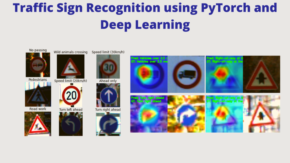
Finally, let’s take a look at some class activation map results.

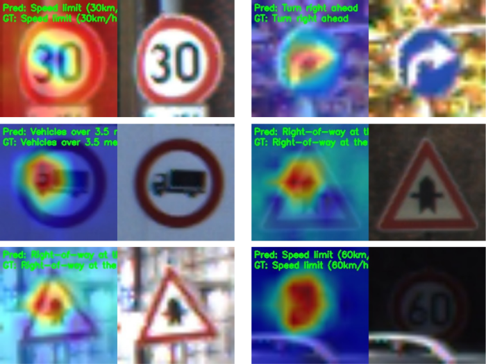
We can see that the model mostly focuses on the center part of each sign for the prediction. This seems correct and also explains why the model may classify a particular image with a particular class.

Further Steps

If you wish to take this project further, you may train different pretrained models like ResNet-18 and even try without pretrained weights. If you find something interesting, then let us know in the comment section.

Summary and Conclusion

In this tutorial, we carried out traffic sign recognition using PyTorch and deep learning with the MobileNetV3 Large model. We saw how to prepare the dataset, how using a learning rate scheduler helps a bit, and also carried out testing with class activation map visualization. In the next post, we will cover traffic sign detection using the Faster RCNN model. I hope that this tutorial was helpful for you.

If you have any doubts, thoughts, or suggestions, then please leave them in the comment section. I will surely address them.

You can contact me using the Contact section. You can also find me on LinkedIn, and Twitter.