
In this tutorial, we will solve an interesting image classification problem. We will train a neural network to recognize real and fake human faces.
Deep Learning has been able to completely transform the field of computer vision. Starting from image classification, object detection, and image segmentation, the applications are unlimited. And since the last few years, image generating GANs (Generative Adversarial Networks) are slowly becoming mainstream in the world of deep learning. GANs in general, are really good at image generation and can generate pretty realistic images too. Nowadays, it can be difficult even for humans to tell apart a real image from one that has been generated by a GAN.

Even though we humans find it difficult to tell whether an image has been generated by a GAN or not, can a deep learning model do it? More importantly, can we train a deep neural network to recognize between real and fake human faces? The answer is YES, and let’s see how to do it in this tutorial.
We will cover the following topics in this tutorial.
- We will start with a brief discussion of image generation capabilities of GANs. As such, we will delve a bit more towards human face generation.
- Then we will move on to discuss what exactly we will be doing in this tutorial.
- Next, checking in with the dataset we will use in this tutorial. This is for training our image classifier.
- Further on, we will discuss the training strategy, hyperparameters, and settings.
- Finally, we will use the trained model to classify some unseen fake and real images of human faces. We will also visualize the class activation maps to know why the model predicted an image as real or fake.
Image Generating Capability of GANs
Since their rise in 2014, GANs nowadays are capable of doing a myriad of things. Most of the applications of GANs fall into the field of computer vision. A few notable ones are:
- Generating realistic looking fake images.
- Image super-resolution.
- Converting paintings to photos and changing weather in photos.
- Creating images out of sketches.
The above cover only a few of them. There are many other applications. And one of the most prominent ones is creating almost life-like images of human faces.
For an instance, let’s take a look at the following images.
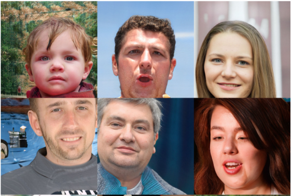
If we show the above images to any person without any context, he or she may say that they look like just any other normal person. But now we know that they are generated by a GAN.
And not just humans, GANs are becoming pretty good at generating images of animals also.
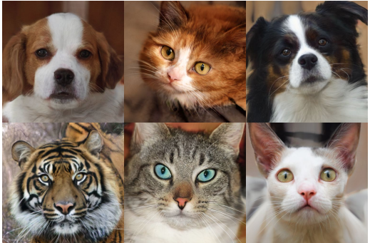
It is just amazing what we can achieve with GANs nowadays.
In any given situation, it will be very difficult for a human being to tell whether the above images are real or a GAN generated them.
But what about a deep learning image classification model? Obviously, just any random model is not of any help to us.
What if we train that model on a few real human faces and fake human faces generated by a GAN? Then we have some hope. Or maybe even better than hope.
That is what we will actually be doing further on in this tutorial.
Approach for this Tutorial
In this tutorial, we train an image classification deep learning on real and fake human faces so that it learns to differentiate between the two.
We will use the Fake-Vs-Real-Faces dataset from Kaggle (more details on this in the next section). Also, we will not train a deep learning model from scratch. That will require way too much data to learn properly. Instead, we will use the MobileNetV3 Large model from Torchvision. We will use the ImageNet weights so that we already get a model which has seen hundreds of thousands of humans already.
We will fine-tune all the layers of the model with a lower learning rate and extensive augmentation. This will introduce ample varying examples to the model to learn well.
One important thing is that we will not go into the image classification code details in this tutorial. The process of image classification is pretty straightforward and the same as what we do in other image classification datasets. But you will get access to all the code, dataset, trained models when you download the zip file for this tutorial.
We will focus on the following things while discussing the training part of the neural network to recognize real and fake human faces:
- The training settings and hyperparameters which include:
- Splitting of the dataset.
- The learning rate.
- Image augmentations.
After training the model, we will also use it for classifying new fake and real images taken from the internet. Along with that, we will also visualize the class activation maps to know exactly why the model thinks an image is real or fake.
The Fake vs Real Human Faces Dataset
We will use the Fake-Vs-Real-Faces dataset to train the neural network to recognize real and fake human faces. The fake faces in this dataset are generated by StyleGan2.
Also, the fake images are collected from the ThisPersonDoesNotExist website. Every time you refresh the page, the GAN will generate a new fake face. And mostly, it will never generate the same fake face twice. For this reason, when testing our model later in the tutorial, we will use a few fake faces from this website.

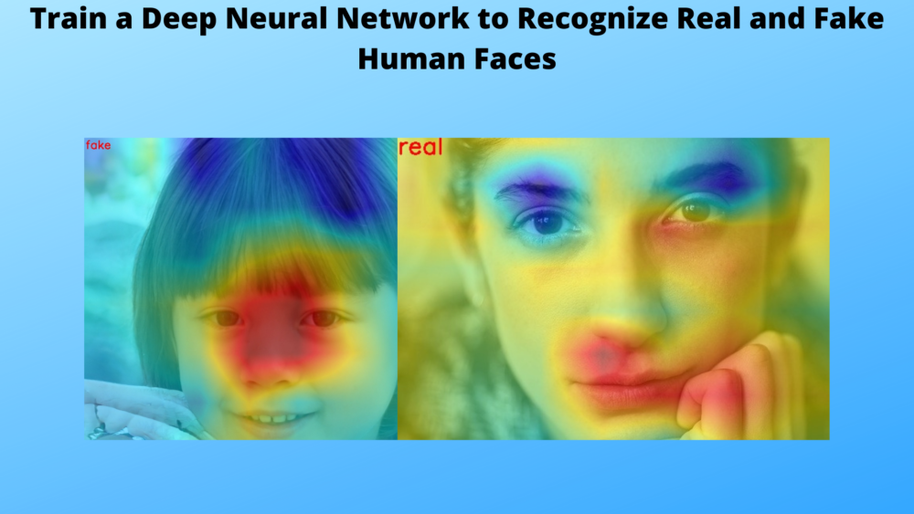
The two above images are from the dataset. Can you tell which is real and which is fake? To be fair, it’s pretty difficult. The human face on the left is the fake one generated by the generator, and the right one is real. This is really difficult for us humans to tell this apart. But as we will see later on, if we train a deep learning model properly, it will be able to distinguish between the two easily.
A few more details about the dataset:
- The dataset contains 1289 images of human faces. Out of these, 700 are fake faces and 589 are real. A bit imbalanced, but nothing much to worry about.
- It has two classes,
fakeandreal. And all the images are in their respective class directories. - All the images have been cropped to 300×300 dimensions.
You can either download the dataset from Kaggle or you can extract the compressed file that you will get access to while downloading the zip file for this tutorial.
Directory Structure
Let’s take a look at the directory structure for the project.
├── input
│   ├── hardfakevsrealfaces
│   │   ├── fake [700 entries exceeds filelimit, not opening dir]
│   │   ├── real [589 entries exceeds filelimit, not opening dir]
│   │   └── data.csv
│   └── test_images
│       ├── fake_image_1.jpeg
│       ├── fake_image_2.jpeg
│       ├── fake_image_3.jpeg
│       ├── real_image_1.jpg
│       ├── real_image_2.jpg
│       └── real_image_3.jpg
├── outputs
│   ├── accuracy.png
│   ├── CAM_fake_image_1.jpg
│   ├── CAM_fake_image_2.jpg
│   ├── CAM_fake_image_3.jpg
│   ├── CAM_real_image_1.jpg
│   ├── CAM_real_image_2.jpg
│   ├── CAM_real_image_3.jpg
│   ├── loss.png
│   └── model.pth
└── src
    ├── cam.py
    ├── datasets.py
    ├── model.py
    ├── train.py
    └── utils.py
- The
inputdirectory contains two subdirectories. Thehardfakevsrealfacessubdirectory contains the class directories and also a CSV file containing the image names and respective labels. We do not need the CSV file for this tutorial. We have all the test images in thetest_imagessubdirectory. These are downloaded from the internet. - Next, we have the
outputdirectory. This contains the trained model, the accuracy & loss graphs, and also the results from running the test script. - Finally, the
srcdirectory contains all the Python code files.
You will get access to all the above files and folders when downloading the zip file for this tutorial. For the dataset, you will get the compressed file that you need to extract before beginning the training.
The PyTorch Version
The code for this tutorial has been developed using PyTorch version 1.10.0. If you wish to install or upgrade PyTorch on your own system, you can do so from the official website.
Training the Neural Network to Recognize Real and Fake Faces
As discussed earlier, we will not go into the coding details of this tutorial. The training code covers a very basic image classification pipeline. You are free to take your time exploring the code after downloading it. We will go over a few important code snippets only.
In the following subsections, we will go over the gist of each Python file and will cover small code snippets wherever needed.
Note that all the Python files are present inside the src directory.
The utils.py Python File
This contains two helper functions, save_model() for saving the trained model, and save_plots() for saving the accuracy and loss graphs.
The datasets.py Python File
The datasets.py creates the training & validation datasets and data loaders for training. We use a 90%/10% split for training and validation. 90% of the data is used for training and 10% for validation. This also applies augmentation to the training set using torchvision.transforms.
Now, there are a few important points regarding the transforms and augmentations. While applying the transforms, we resize the images to 256×256 dimensions. This is larger than the more generic 224×224 resizing while using transfer learning. But this higher resolution will actually help to keep some of the finer features intact in the images. This may help the model to learn better which image is real and which is fake. And from the training experiments, I found that larger resolutions perform better.
Coming to augmentations. We apply random augmentations using the transforms.RandAugment(). More precisely, following is the code snippet for the training transforms.
# Training transforms.
def get_train_transform(RESIZE_TO):
    train_transform = transforms.Compose([
        transforms.Resize((RESIZE_TO, RESIZE_TO)),
        transforms.RandAugment(num_ops=20, magnitude=15),
        transforms.ToTensor(),
        transforms.Normalize(
            mean=[0.485, 0.456, 0.406],
            std=[0.229, 0.224, 0.225]
            )
    ])
    return train_transform
The num_ops argument specifies the number of random augmentations to apply. In our case, the training images will go through 20 random augmentations. With the magnitude argument, we specify the magnitude for all the augmentations that the RandAugment class will apply.
Here, 20 augmentations may seem like a lot. But we most likely need this to build a very robust model. Also, applying so many augmentations may mean that we have to train the model for much longer. Also, note the ImageNet mean and standard deviation values that we are using for normalization. This is because we will be using the MobileNetV3 Large model pretrained on the ImageNet dataset.
The model.py Python File
This file only contains one function, that is, the build_model() function. The function loads the mobilenet_v3_large model from torchvision depending on:
- Whether we want a pretrained model or not.
- Whether to fine-tune all the layers or not.
- The number of classes.
When calling this function, we will be loading the ImageNet pretrained weights, passing the argument to fine-tune all the layers, and providing the number of classes as 2.
The train.py File
The train.py is the executable training script. It combines the elements from all of the above and starts the training. Here are a few important training settings and parameters:
- We have two command line flags, one to control the number of epochs to train for, and the other for the learning rate. We will pass each of these while executing the script.
- When loading the model, we are passing
pretrained=Trueandfine_tune=Trueto load the pretrained weights and fine-tune all the layers. - We are using the Adam optimizer and Cross Entropy loss function.
- After each training epoch, we are printing the training & validation loss and training & validation accuracy.
- In the end, we are saving the trained model and the graphs to disk.
With this, we finish all the information that we need to know about before starting the training. Let’s move on to execute train.py.
Execute train.py
Open your terminal/command line from the src directory and execute the following command.
python train.py --epochs 100 --learning-rate 0.0001
We are training for 100 epochs with a learning rate of 0.0001. This may seem like a lot of epochs for around 1300 images but remember that we are using 20 different augmentations also. So, the model needs to train for longer.
The following is the truncated output from the terminal.
[INFO]: Number of training images: 1161
[INFO]: Number of validation images: 128
[INFO]: Class names: ['fake', 'real']

Computation device: cuda
Learning rate: 0.0001
Epochs to train for: 100

[INFO]: Loading pre-trained weights
[INFO]: Fine-tuning all layers...
4,204,594 total parameters.
4,204,594 training parameters.
[INFO]: Epoch 1 of 100
Training
100%|██████████████████████████████████████████████████████████████████████████████████████████████████████████████████████████████████████████████████████████████████████████████| 73/73 [00:03<00:00, 21.74it/s]
Validation
100%|████████████████████████████████████████████████████████████████████████████████████████████████████████████████████████████████████████████████████████████████████████████████| 8/8 [00:00<00:00, 50.03it/s]


Accuracy of class fake: 100.0
Accuracy of class real: 5.357142857142857


Training loss: 0.518, training acc: 72.524
Validation loss: 0.929, validation acc: 58.594
--------------------------------------------------
[INFO]: Epoch 2 of 100
Training
100%|██████████████████████████████████████████████████████████████████████████████████████████████████████████████████████████████████████████████████████████████████████████████| 73/73 [00:02<00:00, 26.94it/s]
Validation
100%|████████████████████████████████████████████████████████████████████████████████████████████████████████████████████████████████████████████████████████████████████████████████| 8/8 [00:00<00:00, 48.83it/s]


Accuracy of class fake: 100.0
Accuracy of class real: 17.857142857142858


Training loss: 0.315, training acc: 85.530
Validation loss: 1.010, validation acc: 64.062
--------------------------------------------------
...

[INFO]: Epoch 99 of 100
Training
100%|██████████████████████████████████████████████████████████████████████████████████████████████████████████████████████████████████████████████████████████████████████████████| 73/73 [00:02<00:00, 27.08it/s]
Validation
100%|████████████████████████████████████████████████████████████████████████████████████████████████████████████████████████████████████████████████████████████████████████████████| 8/8 [00:00<00:00, 50.67it/s]


Accuracy of class fake: 100.0
Accuracy of class real: 100.0


Training loss: 0.047, training acc: 97.847
Validation loss: 0.006, validation acc: 100.000
--------------------------------------------------
[INFO]: Epoch 100 of 100
Training
100%|██████████████████████████████████████████████████████████████████████████████████████████████████████████████████████████████████████████████████████████████████████████████| 73/73 [00:02<00:00, 26.51it/s]
Validation
100%|████████████████████████████████████████████████████████████████████████████████████████████████████████████████████████████████████████████████████████████████████████████████| 8/8 [00:00<00:00, 46.09it/s]


Accuracy of class fake: 100.0
Accuracy of class real: 100.0


Training loss: 0.048, training acc: 97.588
Validation loss: 0.004, validation acc: 100.000
--------------------------------------------------
TRAINING COMPLETE
The training and validation graphs for accuracy and loss will give even better insights.
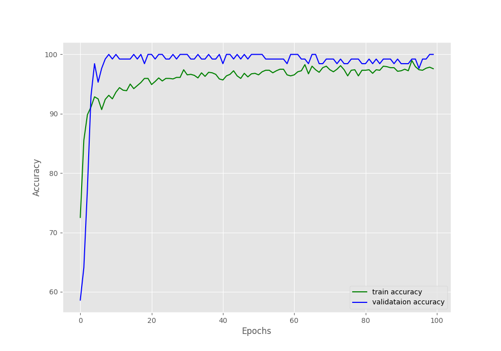
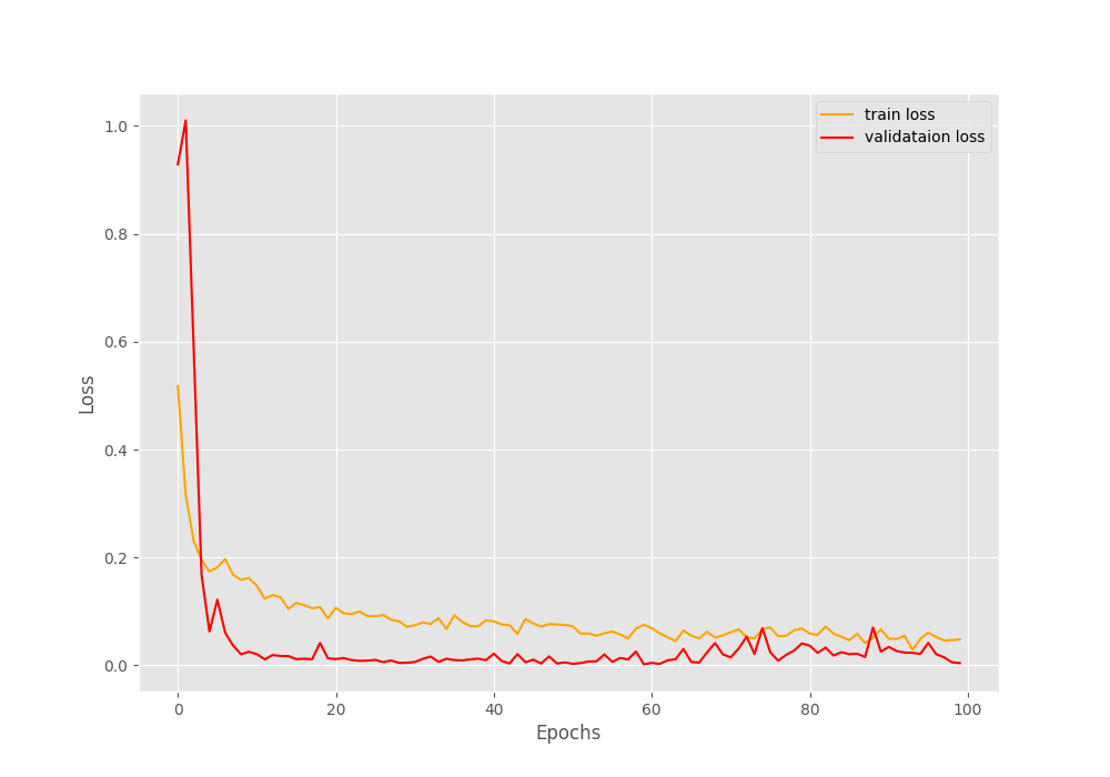
As you can see, because of so many augmentations, even after 100 epochs, the validation results are better than the training results. Obviously, we need to train for longer for the training results to surpass the validation ones.
Still, let’s test our model on new and unseen images and check how it performs.
Testing the Model on New Unseen Images and Visualizing Class Activation Maps
In this section, we will check whether our trained neural network can recognize real and fake human faces. We will feed it some images downloaded from the internet. There are six images in the input/test_images folder. Three are fake human faces and three are real. The naming convention is fake_image_ real_image_ to easily distinguish between them.
The three fake human faces are taken from the thispersondoesnotexist website. We don’t have to worry about testing the model on any images that were already in the training or validation set. Mostly, the GAN that generates the images on the website does generate the same fake faces twice.
Before testing our model, let’s check out one of the fake human faces ourselves and see whether we can find out any way to tell that the image is fake.

The image of the woman above looks astonishingly real in all aspects except one. If we take a look at the lower right lip and fingers we can see some abnormal distortions and blur. We will never find this in a real human face image. The real question here is will the neural network also classify it as fake because of that part of her face?
Let’s check it out.
The cam.py Python File
The cam.py script accomplishes two things. It runs the six test images through the model and also outputs the class activation maps on our custom trained MobileNetV3 Large model.
We are using the code from one of the previous tutorials here. In that tutorial, we trained a custom model to recognize the MNIST Handwritten Digits and visualize class activation maps on new test images. The script in this tutorial will remain almost the same except for the model hook and feature extractor part. That part has been changed to this:
# Hook the feature extractor.
features_blobs = []
def hook_feature(module, input, output):
    features_blobs.append(output.data.cpu().numpy())
model._modules.get('features').register_forward_hook(hook_feature)
# Get the softmax weight
params = list(model.parameters())
weight_softmax = np.squeeze(params[-4].data.cpu().numpy())
The above block shows a part of the code from cam.py. Let’s check out the highlighted lines (5 and 8) in the above code block. The MobileNetV3 Large model has the following structure (truncated for easier understanding):
MobileNetV3(
  (features): Sequential(
    (0): ConvNormActivation(
      (0): Conv2d(3, 16, kernel_size=(3, 3), stride=(2, 2), padding=(1, 1), bias=False)
      (1): BatchNorm2d(16, eps=0.001, momentum=0.01, affine=True, track_running_stats=True)
      (2): Hardswish()
    )
    (1): InvertedResidual(
      (block): Sequential(
        (0): ConvNormActivation(
          (0): Conv2d(16, 16, kernel_size=(3, 3), stride=(1, 1), padding=(1, 1), groups=16, bias=False)
          (1): BatchNorm2d(16, eps=0.001, momentum=0.01, affine=True, track_running_stats=True)
          (2): ReLU(inplace=True)
        )
...
  (avgpool): AdaptiveAvgPool2d(output_size=1)
  (classifier): Sequential(
    (0): Linear(in_features=960, out_features=1280, bias=True)
    (1): Hardswish()
    (2): Dropout(p=0.2, inplace=True)
    (3): Linear(in_features=1280, out_features=2, bias=True)
  )
)
The model has three main blocks, that are, (features), (avgpool), and (classifier). Now, if you observe line 5 in the previous block, we get a hook on the features. On line 8, we get the softmax weights till the AdaptiveAvgPool2d layer.
In the rest of the code, we use these activations to visualize the class activation maps.
Execute cam.py
Execute the following command in the terminal within the src directory.
python cam.py
Let’s check out the class activation maps of the fake images first.
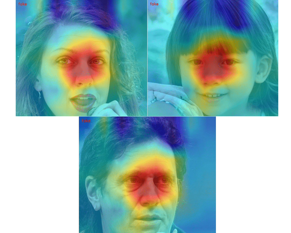
The first thing to note here is that the neural network is able to recognize the fake faces correctly. Now, taking a look at the red regions (high activations) in the images we find something interesting. The model classifies these images as fake based on the eyes, nose, and lower part of the left chin. And it is almost the same for all the fake images. What could be the reason for this?
One of the reasonable explanations for this is that all the three fake images are generated by the same StyleGAN2 model from the same latent distribution. This means that the pixels have some common patterns we as humans cannot see.
To have some more clarity let’s take a look at the class activation maps of the real human faces.
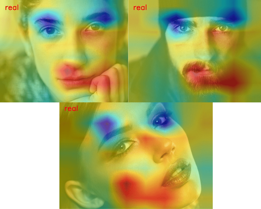
As we can see, the model is able to predict all the real human faces correctly also. Here, apart from the eyes, chin, and cheek, the model is also focusing on the background a bit which it was not doing in the case of the fake images.
If you really want to test the robustness of the model, maybe you can try it on some more fake images generated by a different GAN. If you do so and find some interesting results, let us know in the comment section.
Summary and Conclusion
In this tutorial, we fine-tuned a MobileNetV3 Large neural network model to recognize real and fake human faces. Instead of the classification code, we focused more on the high-level approach and understanding of the project. In the end, we also visualized the class activation maps to know why a model predicts an image as real or fake. I hope that you learned something new from this tutorial.
If you have any doubts, thoughts, or suggestions, please leave them in the comment section. I will surely address them.
You can contact me using the Contact section. You can also find me on LinkedIn, and X.
