
Vision transformers are already good at multiple tasks like image recognition, object detection, and semantic segmentation. However, we can also apply them to data with temporal information like videos. One such use case is using Vision Transformers for video classification. To this end, in this article, we will go over the important parts of the Multiscale Vision Transformer (MViT) paper and also carry out inference using the pretraining model.
Although there are several models for this, the Multiscale Vision Transformer model stands out for video recognition. Along with dealing with temporal data, it also uses multiscale features for video recognition.
We will cover the following topics in this article
- In the first part, we will cover the important sections of the Multiscale Vision Transformer paper.
- First, the drawbacks of other models and approaches.
- Second, the contributions and unique approach of the MViT model.
- Third, the architecture and implementation details of the MViT model.
- Finally, the results on the Kinetics-400 dataset and comparison with other models.
- In the second part, we will code our way through using the MViT model pretrained on the Kinetics-400 dataset for video action recognition.
- Finally, we will discuss some further projects for fine-tuning the Multiscale Vision Transformer model for real-life use cases.
The Multiscale Vision Transformer (MViT) Model
The MViT model was introduced in the paper Multiscale Vision Transformers by researchers from Facebook AI and UC Berkley.
Although simple, the idea is powerful – use multiscale features to train a good video recognition model.
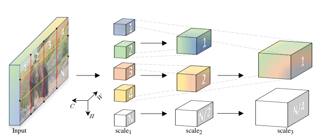
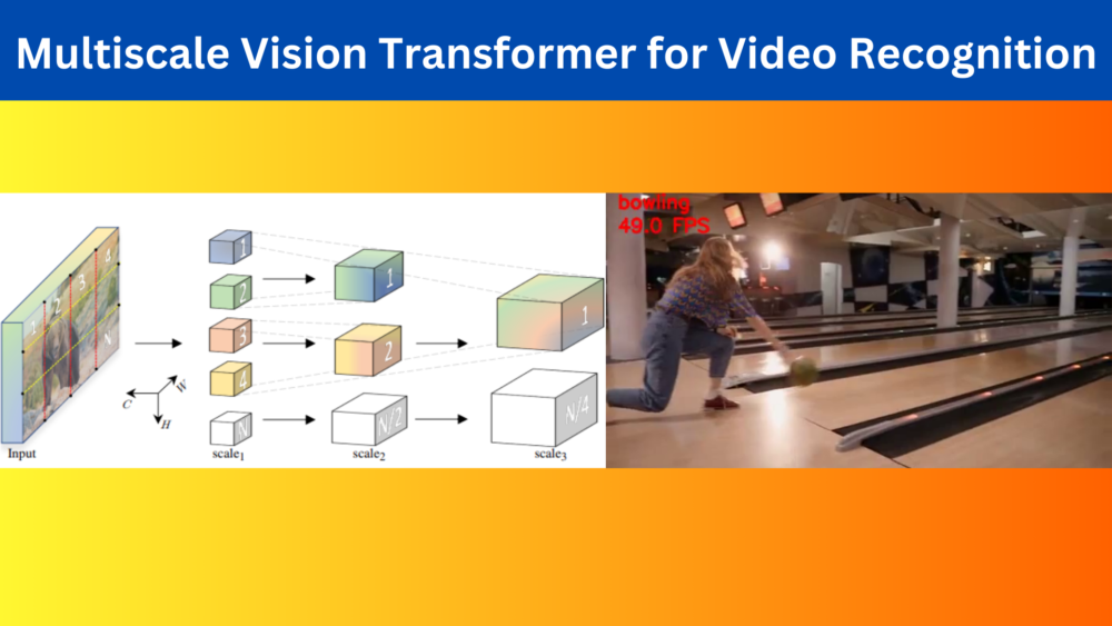
The concept is to build a pyramid of feature hierarchies such that:
- The earlier layers of the MViT model can work on the high resolution spatial resolution to extract the finer features.
- And the lower layers can work on the smaller spatial resolution to extract the course yet complex features.
There is one major drawback of previous models dealing with temporal data and video recognition. In general, transformer neural networks define a constant channel capacity (hidden dimension) throughout the network. This can affect learning features of an image at various levels. MViT tackles the issue from the architecture level.
The MViT Architecture
Following the above idea, the MViT architecture aligns its layers to create a heirarchy of pyramid features.
- It starts with the input image resolution while keeping the channel dimension low.
- Eventually, the layers expand the channel dimension and reduce the spatial resolution, hierarchically.
This provides dense visual concepts to the model along with the fine grained and coarse features. This also leads to the use of temporal information of the video effectively during inference.
As the Multiscale Vision Transformer deals with various resolutions at various stages, the spatial resolution output will vary at each stage.
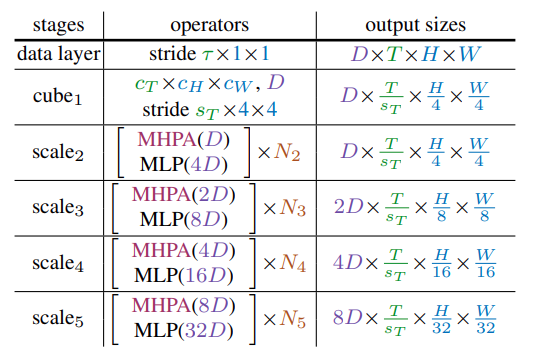
The above figure shows the dimensions (\(D\)) of the Multi-Head Attention and MLP layers at various scales. It also shows the output sizes of the features in the corresponding stages.
We can see that each stage progressively increases the dimension while downsampling the spatial resolution.
Along with architectural changes compared to the original Vision Transformer model, the MViT model also employs various new techniques:
- Pooling operator and pooling attention
- Channel expansion
- Query pooling
I highly recommend going through section 3 of the paper to learn about the above in detail.
Experiments and Results
The authors conduct experiments on various datasets including:
- Kinetics-400 and Kinetics-600
- Something Something v2
- Charades
- AVA
However, we are most interested in the performance on the Kinetics dataset as we will be using a model pretrained on that.
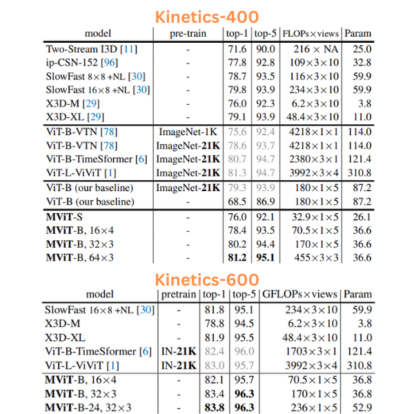
The above figure shows the comparison of Multiscale Vision Transformer with various other models. On the Kinetics-400 dataset, it is easily nearing the performance and even beating some of the ViT based models which have ImageNet pretrained backbones. We can see a similar trend on the Kinetics-600 dataset as well. It is noteworthy because the MViT backbones were not pretrained on the ImageNet dataset.
Furthermore, the parameters of the MViT models are much less compared to the ViT based models. Although it seems that the X3D models are competitive with MViT even with less number of parameters and without pretraining.
In the next section, we will start with the coding part where we will use a pretrained MViT model from Torchvision to run inference on various videos.
Inference using Multiscale Vision Transformer
PyTorch provides a pretrained version of the MViT model. It contains two models, a base model and a small model. We will use the base model which has been trained on the Kinetics-400 dataset. So, it can detect 400 different classes of actions, tasks, and situations from the Kinetics dataset. The dataset is primarily used to train models for action recognition. You may find this GitHub gist helpful to know more about the classes in the dataset.
Let’s take a look at the directory structure before moving forward.
├── input
│   ├── bowling.mp4
│   ├── push_ups.mp4
│   └── welding.mp4
├── outputs
│   ├── barbell_biceps_curl.mp4
│   ├── bowling.mp4
│   ├── chest_fly_machine.mp4
│   ├── push_ups.mp4
│   └── welding.mp4
├── inference_video.py
└── labels.txt
- The
inputdirectory contains the videos that we will use for inference. - The
outputsdirectory contains the inference outputs. - And the parent project directory contains the inference script and a text file containing the class names separated by new lines.
The input files, Python script, and the label text file are downloadable via the download section.
Download Code
Video Inference using MViT
Let’s jump into the code now.
Starting with the import statements and constructing the argument parser.
import torch
import cv2
import argparse
import time
import numpy as np
import os
import albumentations as A
import time

from torchvision.models.video import mvit_v1_b

# Construct the argument parser.
parser = argparse.ArgumentParser()
parser.add_argument(
    '-i', '--input',
    help='path to input video'
)
parser.add_argument(
    '-c', '--clip-len',
    dest='clip_len',
    default=16,
    help='number of frames to consider for each prediction',
    type=int,
)
parser.add_argument(
    '--show',
    action='store_true',
    help='pass to show the video while execution is going on, \
          but requires to uninstall PyAV (`pip uninstall av`)'
)
parser.add_argument(
    '--imgsz',
    default=(256, 256),
    nargs='+',
    type=int,
    help='image resize resolution'
)
parser.add_argument(
    '--crop-size',
    dest='crop_size',
    default=(224, 224),
    nargs='+',
    type=int,
    help='image cropping resolution'
)
args = parser.parse_args()
We need the Albumentations library for carrying out the validation transforms. We also import the mvit_v1_b that we will use to initialize the model.
Let’s go through the different command line flags:
--input: The path to the input video.--clip-len: This is an integer defining the number of video frames that we will feed at a time to the model. It has been trained with a minimum temporal length of 16 frames, so we use that as the default value. The shape of the tensor going into the model during inference will be[batch_size, num_channels, clip_len, height, width]. As we are using RGB video, thenum_channelswill be 3.--show: This is a boolean value indicating that we want to visualize the results on screen during inference.--imgszand--crop-size: The image size for resizing and final crop size. This also follows the training hyperparameters where the input image was first resized to 256×256 resolution and cropped to 224×224.
Considering the default values, the shape of the tensor going into the model will be [1, 3, 16, 224, 225].
Next, let’s create the output directory, define the transforms, and load the MViT model.
OUT_DIR = os.path.join('outputs')
os.makedirs(OUT_DIR, exist_ok=True)

# Define the transforms.
crop_size = tuple(args.crop_size)
resize_size = tuple(args.imgsz)
transform = A.Compose([
    A.Resize(resize_size[1], resize_size[0], always_apply=True),
    A.CenterCrop(crop_size[1], crop_size[0], always_apply=True),
    A.Normalize(
        mean=[0.45, 0.45, 0.45],
        std=[0.225, 0.225, 0.225],
        always_apply=True
    )
])

#### PRINT INFO #####
print(f"Number of frames to consider for each prediction: {args.clip_len}")
print('Press q to quit...')

device = torch.device('cuda' if torch.cuda.is_available() else 'cpu')

# Load the model.
model = mvit_v1_b(weights='DEFAULT').to(device).eval()

# Load the labels file.
with open('labels.txt', 'r') as f:
    class_names = f.readlines()
    f.close()
Do note use mean and standard deviation values as explained in the official PyTorch documentation.
We are loading the Multiscale Vision Transformer model with the default weights which will automatically choose the best pretrained weights.
We read the labels file and store them in class_names.
Now, we need to read the video file and initialize the rest of the variables.
# Get the frame width and height.
frame_width = int(cap.get(3))
frame_height = int(cap.get(4))
fps = int(cap.get(5))

save_name = f"{args.input.split('/')[-1].split('.')[0]}"
# Define codec and create VideoWriter object.
out = cv2.VideoWriter(
    f"{OUT_DIR}/{save_name}.mp4",
    cv2.VideoWriter_fourcc(*'mp4v'),
    fps,
    (frame_width, frame_height)
)

frame_count = 0 # To count total frames.
total_fps = 0 # To get the final frames per second.

# A clips list to append and store the individual frames.
clips = []
The clips list will be used to store the temporal frames, 16 in our case.
Finally, looping over the video frames and carrying out the inference.
# Read until end of video.
while(cap.isOpened()):
    # Capture each frame of the video.
    ret, frame = cap.read()
    if ret == True:
        # Get the start time.
        start_time = time.time()

        image = frame.copy()
        frame = cv2.cvtColor(frame, cv2.COLOR_BGR2RGB)
        frame = transform(image=frame)['image']
        clips.append(frame)

        if len(clips) == args.clip_len:
            input_frames = np.array(clips)
            # Add an extra dimension        .
            input_frames = np.expand_dims(input_frames, axis=0)
            # Transpose to get [1, 3, num_clips, height, width].
            input_frames = np.transpose(input_frames, (0, 4, 1, 2, 3))
            # Convert the frames to tensor.
            input_frames = torch.tensor(input_frames, dtype=torch.float32)
            input_frames = input_frames.to(device)

            with torch.no_grad():
                outputs = model(input_frames)

            # Get the prediction index.
            _, preds = torch.max(outputs.data, 1)

            # Map predictions to the respective class names.
            label = class_names[preds].strip()

            # Get the end time.
            end_time = time.time()
            # Get the fps.
            fps = 1 / (end_time - start_time)
            # Add fps to total fps.
            total_fps += fps
            # Increment frame count.
            frame_count += 1
            print(f"Frame: {frame_count}, FPS: {fps:.1f}")

            cv2.putText(
                image,
                label,
                (15, 25),
                cv2.FONT_HERSHEY_SIMPLEX,
                0.8,
                (0, 0, 255),
                2,
                lineType=cv2.LINE_AA
            )
            cv2.putText(
                image,
                f"{fps:.1f} FPS",
                (15, 55),
                cv2.FONT_HERSHEY_SIMPLEX,
                0.8,
                (0, 0, 255),
                2,
                lineType=cv2.LINE_AA
            )

            clips.pop(0)

            if args.show:
                cv2.imshow('image', image)
                # Press `q` to exit.
                if cv2.waitKey(1) & 0xFF == ord('q'):
                    break
            out.write(image)
    else:
        break

# Release VideoCapture().
cap.release()
# Close all frames and video windows.
cv2.destroyAllWindows()
# Calculate and print the average FPS.
avg_fps = total_fps / frame_count
print(f"Average FPS: {avg_fps:.3f}")
Forward Pass Note
The only major part to note here starts from line 108. We do not start the forward pass until we have 16 frames in the clips list. We convert the entire list into a NumPy array and apply further preprocessing of transposing and converting them to PyTorch tensors.
Then we forward an entire batch containing 16 frames thgrough the model, predict the class name, calculate the FPS, and annotate the current frame with the FPS and the class name.
Finally, we visualize the frame on the screen and store the result to disk.
Executing the Video Inference Script
While executing, we need to provide the path to the input file as a mandatory argument.
Let’s start with a bowling video.
python inference_video.py --input input/bowling.mp4 --show
The results are quite good. The model can predict the action correctly in all the frames.
Next, let’s try another activity.
python inference_video.py --input input/welding.mp4 --show
Here also, the model can detect the welding action correctly.
Finally, let’s try a video where the model performs poorly.
python inference_video.py --input input/push_ups.mp4 --show
In this case, the model is failing whenever is person is at the extreme top or bottom. It’s rather difficult to pinpoint why that might be. It may happen that the model not getting enough information for that period of time when the person is pausing.
Some Real Life Use Cases of Fine-Tuning Video Action Recognition Models
There are several cases where we may want to fine-tune a video action recognition model.
These include:
- Sports analytics
- Surveillance and monitoring
- Healthcare monitoring
We will try to tackle these use cases in future articles.
Further Reading
- Action Recognition in Videos using Deep Learning and PyTorch
- Train S3D Video Classification Model using PyTorch
- Training a Video Classification Model from Torchvision
Summary and Conclusion
In this article, we discussed the Multiscale Vision Transformer model including its contribution, architecture, and also running inference on videos. We analyzed the results and found that the model may be falling behind in some action recognition tasks. We also discussed some use cases where we can fine-tune such action recognition models. I hope that this article was worth your time.
If you have any doubts, thoughts, or suggestions, please leave them in the comment section. I will surely address them.
You can contact me using the Contact section. You can also find me on LinkedIn, and X.
Acknowledgment
