Training a Video Classification Model from Torchvision

Video classification is an important task in computer vision and deep learning. Although very similar to image classification, the applications are far more impactful. Starting from surveillance to custom sports analytics, the use cases are vast. When starting with video classification, mostly we train a 2D CNN model and use average rolling predictions while running inference on videos. However, there are 3D CNN models for such tasks. This article will cover a simple pipeline for training a video classification model from Torchvision on a custom dataset.

Most of the video classification models in Torchvision are pretrained on a vast amount of data. These are mostly different versions of the Kinetics dataset. But we will choose a far smaller set of training data here. This will make us comfortable with the entire pipeline of video classification using a custom dataset.

Before moving into the technical parts, here are the points that we will cover in the article:

• We will start with the exploration of the training dataset. We will use a subset of the UCF50 dataset for training our Torchvision video classification model.
• The next part is the discussion of the code. Mainly, we will focus on the model and the training pipeline.
• After training, we will use various videos from the internet and run inference using the best weights from the training.

NOTE: We will skip some technical parts because we want to focus entirely on the model and training script. These include the dataset preparation code and the utilities. However, all the code will be available for download and use in your own projects.

The UCF50 Dataset for Training Video Classification Model using Torchvision

Video classification training is expensive in terms of required GPU computing. So, we have to choose a small dataset to train the model. UCF50 is a perfect dataset for this. As a lot of the classes from the dataset match with the Kinetics dataset on which all of the Torchvision video classification models are trained, we do not have to worry about accuracy. We can entirely focus on learning the ropes of video classification.

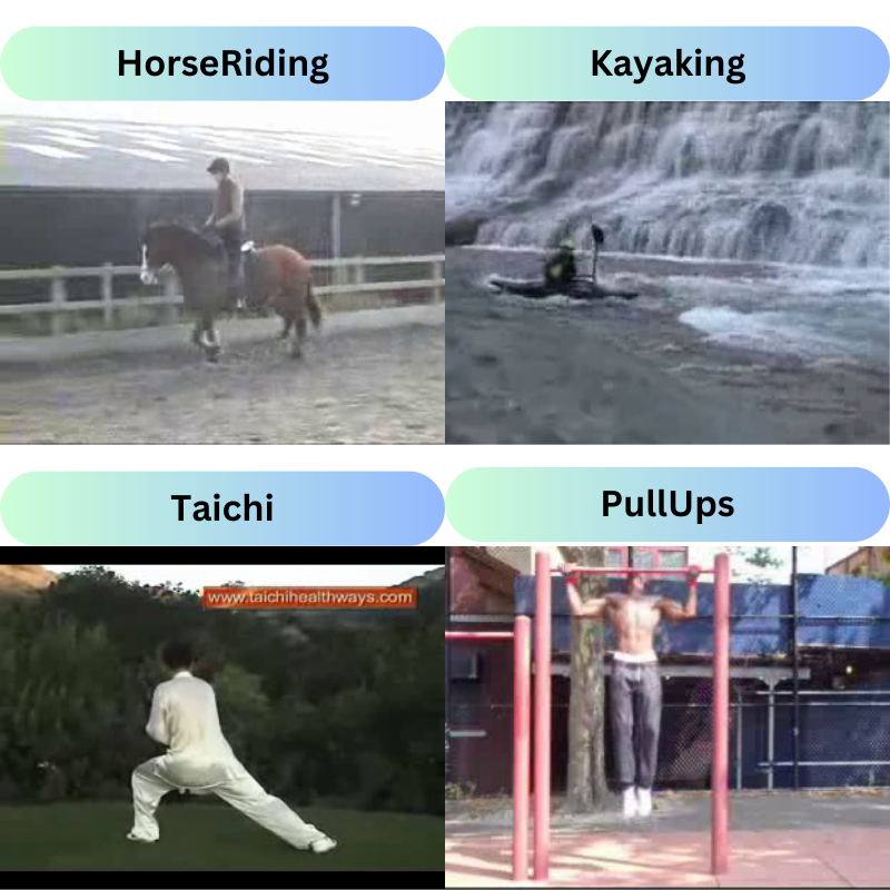
The UCF50 dataset contains action recognition videos from YouTube belonging to 50 categories. These include videos in various lighting conditions, cluttered backgrounds, and even different camera motions.

You can go ahead and download the UCF50 dataset from here.

After downloading and extracting the dataset, you will see the following structure.

# This shows truncated directory structure.
UCF50
├── BaseballPitch
...
├── TennisSwing
├── ThrowDiscus
├── TrampolineJumping
├── VolleyballSpiking
├── WalkingWithDog
└── YoYo

There are 50 directories each indicating the class name. All these directories contain around 100 to 200 short video clips belonging to that class.

For example, here is a clip from the YoYo directory.

As we will be using a pretrained model, we will not need all the videos from each class. We will use a subset for training. Also, we will create a validation split. We will come to this later while discussing the coding parts of the article.

If you wish to run the training experiments on your system, please go ahead and download the dataset.

Project Directory Structure

Let’s take a look at the directory structure of the entire project.

├── input
│   ├── inference_data
│   ├── UCF50
│   └── ucf50_train_valid
├── outputs
│   ├── inference
│   ├── accuracy.png
│   ├── best_model.pth
│   ├── loss.png
│   └── model.pth
└── src
    ├── class_names.py
    ├── datasets.py
    ├── inference_video.py
    ├── model.py
    ├── presets.py
    ├── split_ucf50.py
    ├── train.py
    └── utils.py

• The input directory contains the original UCF50 dataset and the one with the training and validation split that we will use for training. Later will see how to create this split.
• The outputs directory contains the training and inference outputs.
• In the src directory, we have all the Python files that will be used for training and inference. In this article, we will mostly focus on the train.py and model.py files.

All the Python files, pretrained weights, and inference videos are available via the download section of this article. In case you want to train the model, you will need to download the UCF50 dataset.

PyTorch Version and Other Dependencies

The code for this article uses PyTorch 2.0.1. But any PyTorch version starting from 1.12.1 should work without issues.

Another major dependency for the data loading part is PyAV. We need this for the dataset preparation when running the training script. You can install it using the following command:

pip install av

However, this library causes a major issue during inference. The OpenCV’s imshow() does not work when PyAV is installed and we have to uninstall it before running inference. We will talk more about this in the inference section.

Training Torchvision Video Classification Model

Let’s start with the interesting part of the article, getting into the code.

For most of the data loading part, we are adapting the official Torchvision video classification scripts. But I have modified and simplified most of the code for only the parts that we need here. The rest of the scripts, like training and inference are custom code to facilitate easier understanding.

Download Code

Creating the Train and Validation Split of The UCF50 Dataset

For training the Torchvision video classification model, first, we have to create a train/validation split of the dataset.

The split_ucf50.py file contains a simple script to do so. 10% of the dataset will be used for validation and 90% is reserved for training.

But we are not using the entire 90% for training the model here. It contains a TRAINING_PERCENTAGE control factor that accepts a value between 0.0 to 1.0. This defines the percentage of data to use for training out of 90%. By default, it is set to 0.35 indicating that only 35% of the 90% data will be used to create the training set.

We can execute the following command to create the split.

python split_ucf50.py 

100%|██████████████████████████████████| 2104/2104 [00:00<00:00, 4096.41it/s]
100%|██████████████████████████████████| 669/669 [00:00<00:00, 3953.44it/s] 

From the above output, we can see that there are 2104 videos for training and 669 videos for validation across all 50 classes.

The new split data is in the input/ucf50_train_valid directory.

Video Classification Training Dataset Preparation in Brief

The datasets.py and presets.py files contain all the code that we need to prepare the data for training the video classification model.

The presets.py file contains the transforms and augmentations that we will apply to the video frames. Here, we use a mean of (0.43216, 0.394666, 0.37645) and a standard deviation of (0.22803, 0.22145, 0.216989). These two match that of the Kinetics-400 dataset as we will be using a model pretrained on this dataset.

Further, we also apply a simple horizontal flip augmentation to the frames with 0.5 probability. This will ensure that the video classification model does not overfit too soon.

Moving ahead, the entirety of the Video Classification dataset preparation code is in the datasets.py file. While preparing the video frames, first we will be resizing them to 128×171 resolution, and applying Random Crop to make them 112×112 resolution. These values are defined in the train.py script before we create the dataset instances.

The Video Classification Model

For our experiments, we will use the MC3_18 video classification model. This has been pretrained on the Kinetics-400 dataset. As such, we can directly use the model for human action recognition. But here, our objective is to use this for transfer learning. So, let’s modify the model.

This model is like an 18-layer Residual Neural Network but with 3D convolutions instead of 2D convolutions.

Here is the code for preparing the model that is present in the model.py file.

from torchvision import models

import torch.nn as nn

def build_model(fine_tune=True, num_classes=10):
    model = models.video.mc3_18(weights='DEFAULT')
    if fine_tune:
        print('[INFO]: Fine-tuning all layers...')
        for params in model.parameters():
            params.requires_grad = True
    if not fine_tune:
        print('[INFO]: Freezing hidden layers...')
        for params in model.parameters():
            params.requires_grad = False
    model.fc = nn.Linear(in_features=512, out_features=num_classes)
    return model

if __name__ == '__main__':
    model = build_model()
    print(model)
    # Total parameters and trainable parameters.
    total_params = sum(p.numel() for p in model.parameters())
    print(f"{total_params:,} total parameters.")
    total_trainable_params = sum(
        p.numel() for p in model.parameters() if p.requires_grad)
    print(f"{total_trainable_params:,} training parameters.")

We have a build_model() function that accepts two parameters, fine_tune and num_classes. The first one will decide whether we want to fine-tune the model or just use transfer learning by training the classification head only. The latter defines the number of classes in the classification head.

For our purpose, we need to modify the final classification layer of the MC3_18 video classification model. This is the same as any other image classification model. We define a linear layer with the out_features matching the number of classes in the dataset.

Note: We are not going in-depth into the model architecture here. We will understand several video classification models in detail in future posts.

The Training Script for the Video Classification Model

The training script is quite important for video classification. It contains a lot of intricacies particular to the video classification dataset preparation and metric. Let’s go through it in detail.

All the code for this is present in the train.py file.

The following code block defines the import statements and sets the seed for reproducibility.

import torch
import argparse
import torch.nn as nn
import torch.optim as optim
import os
import numpy as np
import random
import presets

from tqdm.auto import tqdm
from model import build_model
from datasets import VideoClassificationDataset
from utils import save_model, save_plots, SaveBestModel
from class_names import class_names
from torchvision.datasets.samplers import (
    RandomClipSampler, UniformClipSampler
)
from torch.utils.data.dataloader import default_collate

seed = 42
np.random.seed(seed)
random.seed(seed)
torch.manual_seed(seed)
torch.cuda.manual_seed(seed)
torch.cuda.manual_seed_all(seed)
torch.backends.cudnn.deterministic = True 

There are two important imports in the above block. In video classification, we need the RandomClipSampler, and the UniformSampler.

The sampling of video frames in this case is quite different than what we do in image classification. We will discuss more about these two classes in detail when preparing the dataset instances.

Next, we have quite a few argument parsers for the command line that we can pass while executing the script.

# Construct the argument parser.
parser = argparse.ArgumentParser()
parser.add_argument(
    '-e', '--epochs', 
    type=int, 
    default=10,
    help='Number of epochs to train our network for'
)
parser.add_argument(
    '-lr', '--learning-rate', 
    type=float,
    dest='learning_rate', 
    default=0.001,
    help='Learning rate for training the model'
)
parser.add_argument(
    '-b', '--batch-size',
    dest='batch_size',
    default=32,
    type=int
)
parser.add_argument(
    '-ft', '--fine-tune',
    dest='fine_tune' ,
    action='store_true',
    help='pass this to fine tune all layers'
)
parser.add_argument(
    '--save-name',
    dest='save_name',
    default='model',
    help='file name of the final model to save'
)
parser.add_argument(
    '--scheduler',
    action='store_true',
    help='use learning rate scheduler if passed'
)
parser.add_argument(
    '--workers', 
    default=4,
    help='number of parallel workers for data loader',
    type=int
)
args = parser.parse_args()

Some of the important arguments from the above block are:

• --fine-tune: This is a boolean argument indicating whether we want to fine-tune the entire model or just train the new classification head.
• --workers: This is the number of parallel workers that will be used for dataset preparation. This will be used during both, the parsing of the video frames when creating the dataset instances and also for the data loaders during training. A higher number of workers can save a few seconds on each training epoch but also require more RAM.

Training, Validation, and Collate Functions

Apart from the training and validation functions, we also need a collation function.

def collate_fn(batch):
    batch = [(d[0], d[1]) for d in batch]
    return default_collate(batch)

It receives a batch of data and returns only the video frames and their respective labels. This is helpful when the __getitem__() method returns metadata along with the frames and labels.

Next are the training and validation functions. Let’s take a closer look at them.

# Training function.
def train(model, trainloader, optimizer, criterion):
    model.train()
    print('Training')
    train_running_loss = 0.0
    train_running_correct = 0
    bs_accumuator = 0
    counter = 0
    prog_bar = tqdm(
        trainloader, 
        total=len(trainloader), 
        bar_format='{l_bar}{bar:20}{r_bar}{bar:-20b}'
    )
    for i, data in enumerate(prog_bar):
        counter += 1
        image, labels = data
        image = image.to(device)
        labels = labels.to(device)
        optimizer.zero_grad()
        # Forward pass.
        outputs = model(image)
        bs_accumuator += outputs.shape[0]
        # Calculate the loss.
        loss = criterion(outputs, labels)
        train_running_loss += loss.item()
        # Calculate the accuracy.
        _, preds = torch.max(outputs.data, 1)
        
        train_running_correct += (preds == labels).sum().item()
        # Backpropagation.
        loss.backward()
        # Update the weights.
        optimizer.step()
    # Loss and accuracy for the complete epoch.
    epoch_loss = train_running_loss / counter
    epoch_acc = 100. * (train_running_correct / bs_accumuator)
    return epoch_loss, epoch_acc

The train() function looks a lot like an image classification training function but with one major change. We calculate the clip-wise accuracy here instead of video accuracy. Therefore, we have a bs_accumulator which keeps on incrementing by the value of batch size on each iteration. Finally, we divide the total number of correct predictions by the bs_accumulator to get the epoch-wise accuracy.

The validate() function follows a similar structure.

# Validation function.
def validate(model, testloader, criterion):
    model.eval()
    print('Validation')
    valid_running_loss = 0.0
    valid_running_correct = 0
    bs_accumuator = 0
    counter = 0
    prog_bar = tqdm(
        testloader, 
        total=len(testloader), 
        bar_format='{l_bar}{bar:20}{r_bar}{bar:-20b}'
    )
    with torch.no_grad():
        for i, data in enumerate(prog_bar):
            counter += 1
            
            image, labels = data
            image = image.to(device)
            labels = labels.to(device)
            # Forward pass.
            outputs = model(image)
            bs_accumuator += outputs.shape[0]
            # Calculate the loss.
            loss = criterion(outputs, labels)
            valid_running_loss += loss.item()
            # Calculate the accuracy.
            _, preds = torch.max(outputs.data, 1)
            valid_running_correct += (preds == labels).sum().item()
        
    # Loss and accuracy for the complete epoch.
    epoch_loss = valid_running_loss / counter
    epoch_acc = 100. * (valid_running_correct / bs_accumuator)
    return epoch_loss, epoch_acc

We do not need backpropagation or the optimizer update step during validation.

The Main Block

The main code block (if __name__ == '__main__') is also quite essential while doing video classification training for the first time. To avoid confusion and adhere to the indentation, here is the entire code block.

if __name__ == '__main__':
    # Create a directory with the model name for outputs.
    out_dir = os.path.join('..', 'outputs')
    os.makedirs(out_dir, exist_ok=True)

    #### TRANSFORMS ####
    train_crop_size = (112, 112)
    train_resize_size = (128, 171)

    transform_train = presets.VideoClassificationPresetTrain(
        crop_size=train_crop_size, 
        resize_size=train_resize_size
    )
    transform_valid = presets.VideoClassificationPresetTrain(
        crop_size=train_crop_size, 
        resize_size=train_resize_size, 
        hflip_prob=0.0
    )

    # Load the training and validation datasets.
    dataset_train = VideoClassificationDataset(
        '../input/ucf50_train_valid',
        frames_per_clip=16,
        frame_rate=15,
        split="train",
        transform=transform_train,
        extensions=(
            "mp4",
            'avi'
        ),
        output_format="TCHW",
        num_workers=args.workers
    )
    dataset_valid = VideoClassificationDataset(
        '../input/ucf50_train_valid',
        frames_per_clip=16,
        frame_rate=15,
        split="valid",
        transform=transform_valid,
        extensions=(
            "mp4",
            'avi'
        ),
        output_format="TCHW",
        num_workers=args.workers
    )
    print(f"[INFO]: Number of training images: {len(dataset_train)}")
    print(f"[INFO]: Number of validation images: {len(dataset_valid)}")
    print(f"[INFO]: Classes: {class_names}")


    # Load the training and validation data loaders.
    train_sampler = RandomClipSampler(
        dataset_train.video_clips, max_clips_per_video=5
    )
    test_sampler = UniformClipSampler(
        dataset_valid.video_clips, num_clips_per_video=5
    )
    train_loader = torch.utils.data.DataLoader(
        dataset_train,
        batch_size=args.batch_size,
        sampler=train_sampler,
        num_workers=args.workers,
        pin_memory=True,
        collate_fn=collate_fn,
    )
    valid_loader = torch.utils.data.DataLoader(
        dataset_valid,
        batch_size=args.batch_size,
        sampler=test_sampler,
        num_workers=args.workers,
        pin_memory=True,
        collate_fn=collate_fn,
    )

    # Learning_parameters. 
    lr = args.learning_rate
    epochs = args.epochs
    device = ('cuda' if torch.cuda.is_available() else 'cpu')
    print(f"Computation device: {device}")
    print(f"Learning rate: {lr}")
    print(f"Epochs to train for: {epochs}\n")

    # Load the model.
    model = build_model(
        fine_tune=args.fine_tune, 
        num_classes=50
    ).to(device)
    print(model)
    
    # Total parameters and trainable parameters.
    total_params = sum(p.numel() for p in model.parameters())
    print(f"{total_params:,} total parameters.")
    total_trainable_params = sum(
        p.numel() for p in model.parameters() if p.requires_grad)
    print(f"{total_trainable_params:,} training parameters.")

    # Optimizer.
    optimizer = torch.optim.SGD(
        model.parameters(), 
        lr=lr, 
        momentum=0.9, 
    )
    # Loss function.
    criterion = nn.CrossEntropyLoss()

    # Initialize `SaveBestModel` class.
    save_best_model = SaveBestModel()

    # LR scheduler.
    scheduler = optim.lr_scheduler.MultiStepLR(
        optimizer, milestones=[7], gamma=0.1, verbose=True
    )

    # Lists to keep track of losses and accuracies.
    train_loss, valid_loss = [], []
    train_acc, valid_acc = [], []
    # Start the training.
    for epoch in range(epochs):
        print(f"[INFO]: Epoch {epoch+1} of {epochs}")
        train_epoch_loss, train_epoch_acc = train(
            model, train_loader, optimizer, criterion
        )
        valid_epoch_loss, valid_epoch_acc = validate(
            model, valid_loader, criterion
        )
        train_loss.append(train_epoch_loss)
        valid_loss.append(valid_epoch_loss)
        train_acc.append(train_epoch_acc)
        valid_acc.append(valid_epoch_acc)
        print(f"Training loss: {train_epoch_loss:.3f}, training acc: {train_epoch_acc:.3f}")
        print(f"Validation loss: {valid_epoch_loss:.3f}, validation acc: {valid_epoch_acc:.3f}")
        save_best_model(
            valid_epoch_loss, epoch, model, out_dir, args.save_name
        )
        if args.scheduler:
            scheduler.step()
        print('-'*50)

    # Save the trained model weights.
    save_model(epochs, model, optimizer, criterion, out_dir, args.save_name)
    # Save the loss and accuracy plots.
    save_plots(train_acc, valid_acc, train_loss, valid_loss, out_dir)
    print('TRAINING COMPLETE')

• On lines 152 and 153, we define the crop size and resize resolution. We use this for both training and validation transform preparation on lines 155 and 159.
• Moving ahead, we create the training and validation datasets on lines 166 and 179. Here, the frames_per_clip argument defines how many frames we want to extract from each clip. Also, the frame_rate defines the number of frames per second (FPS) of the extracted clip. This remains the same for both datasets.
• From the above point, it is clear that we extract multiple clips from each video. We define this on lines 198 and 201. We use the RandomClipSampler for training and UniformClipSampler for validation. The former accepts max_clips_per_video which we give as 5. This means that 5 clips will be extracted at random intervals from each video. The latter accepts num_clips_per_video which we also pass as 5. This will serially extract 5 clips of 16 frames from each video.
• Then we define the data loaders just as in the case of any other PyTorch training process.
• Next, we define the learning rate, the number of epochs, and the computation device.
• While preparing the model, we pass whether we want to fine-tune the model or not.
• We are using the SGD optimizer with a momentum of 0.9.
• The training loop starts on line 264 and we try to save the best model after each epoch based on the least loss.

We also save the accuracy and loss plots at the end.

This is all we have for the training script. Let’s train and model and analyze its performance.

Training the Video Classification Model

Note: All the training and inference experiments were run on a machine with 10 GB RTX 3080 GPU, 10th generation i7 CPU, and 32 GB of RAM.

We can execute the following command to start the training process.

python -W ignore train.py --epochs 20 --workers 10 --batch-size 32

The -W ignore helps ignore warnings from the video reading script of PyTorch.

We are training the model for 20 epochs with 10 parallel workers for data loading and a batch size of 32. Please adjust the configuration according to your hardware in case you carry out training. As you may see, we are not passing the --fine-tune argument. So, we are training just the final classification layer.

Here are the truncated outputs.

[INFO]: Freezing hidden layers...
VideoResNet(
  (stem): BasicStem(
    (0): Conv3d(3, 64, kernel_size=(3, 7, 7), stride=(1, 2, 2), padding=(1, 3, 3), bias=False)
    (1): BatchNorm3d(64, eps=1e-05, momentum=0.1, affine=True, track_running_stats=True)
    (2): ReLU(inplace=True)
  )
.
.
.
11,515,890 total parameters.
25,650 training parameters.
Adjusting learning rate of group 0 to 1.0000e-03.
[INFO]: Epoch 1 of 20
Training
100%|████████████████████| 329/329 [01:19<00:00,  4.14it/s]                                                                                                                                   
Validation
100%|████████████████████| 105/105 [00:27<00:00,  3.78it/s]                                                                                                                                   
Training loss: 2.699, training acc: 53.376
Validation loss: 1.638, validation acc: 80.927

Best validation loss: 1.638469544478825

Saving best model for epoch: 1

--------------------------------------------------
.
.
.
[INFO]: Epoch 20 of 20
Training
100%|████████████████████| 329/329 [01:19<00:00,  4.16it/s]                                                                                                                                   
Validation
100%|████████████████████| 105/105 [00:28<00:00,  3.63it/s]                                                                                                                                   
Training loss: 0.182, training acc: 97.480
Validation loss: 0.238, validation acc: 95.187

Best validation loss: 0.23800168679805384

Saving best model for epoch: 20

--------------------------------------------------
TRAINING COMPLETE

We can observe that we are training just 25,650 parameters in the entire model. We freeze all other layers and rely upon the pretrained weights for the performance of the model.

Astonishingly, the model was improving till the final epoch of training. In the last epoch, the validation loss was 0.23 where the best model was saved. Further, the MC3_18 video classification model reached a validation accuracy of 95.187% which is quite high considering we are training only the final layers.

To get a better idea, here are the accuracy and loss plots.

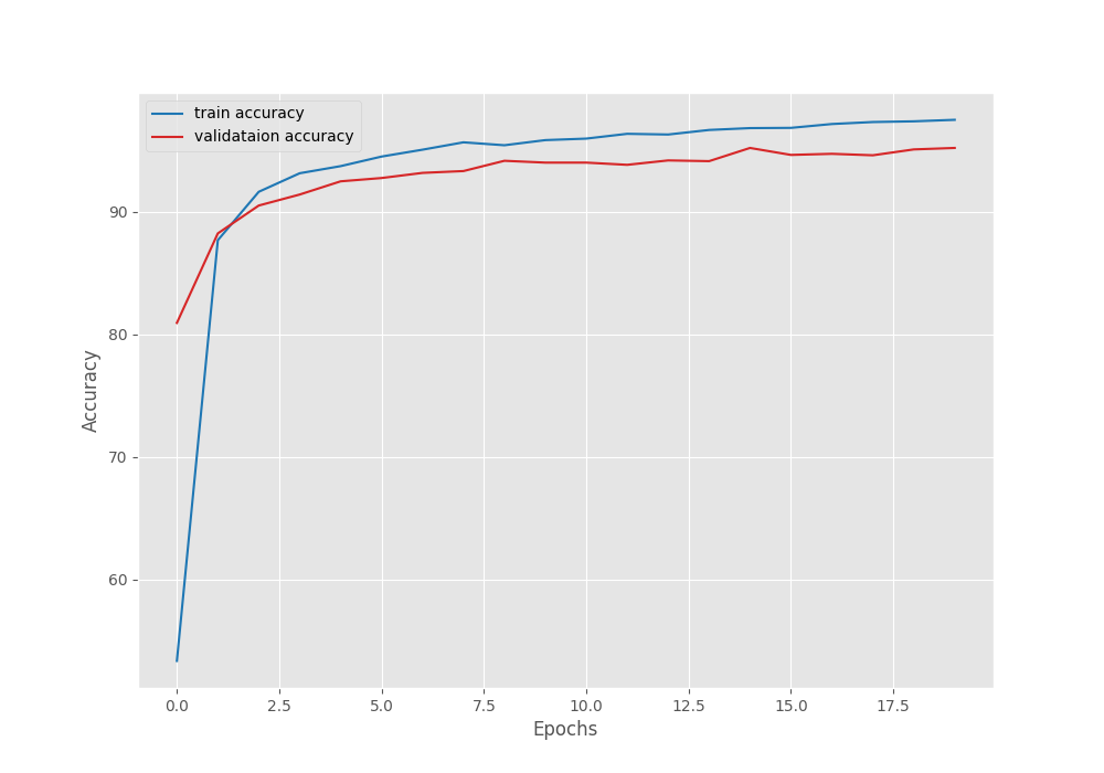
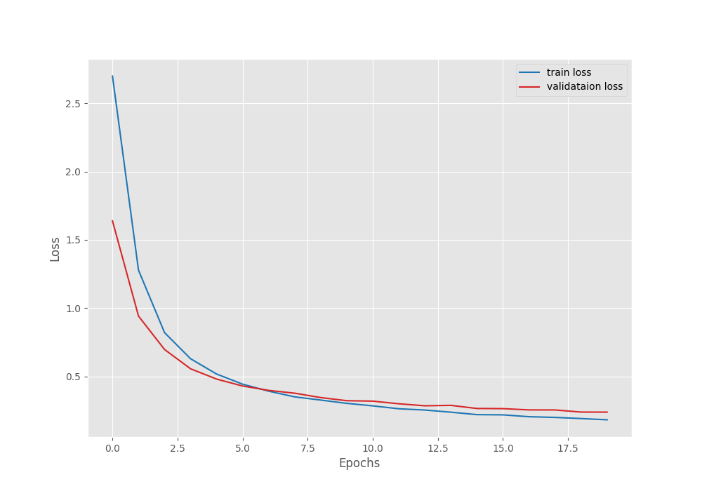
It is clear that the model was still improving. Most probably, we can train it for a few more epochs to get an even better model. And all this just by training the final layers and using only 35% of the training data.

Inference on Unseen Videos using the Trained MC3_18 Video Classification Model

The inference_video.py script contains the code for running video classification inference. You can find a detailed explanation of how the code works in the Human Action Recognition post. The post goes into a lot of detail about the working of the video classification models in PyTorch.

Here, we will just run the inference.

Note: Please uninstall PyAV using the following command before running inference as it causes video visualization issues using OpenCV.

pip uninstall av

We can run the following command to start our inference experiments.

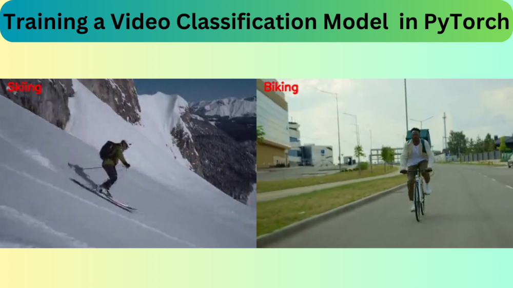
python inference_video.py --input ../input/inference_data/biking.mp4

The results are perfect here. The model predicted all the frames correctly.

Here are two more results whose video files you can find in the input/inference_data directory. You can just change the --input path argument and run inference on the following videos.

The predictions in both the resulting videos are correct in all the frames.

However, here is a video of billiards on which the model does not perform very well. This video is available in the inference data directory as well.

The model predicts the class correctly in a few frames only. Most probably we can improve the results by using more training data, with longer training, or even fine-tuning all the layers of the MC3_18 video classification model.

Summary and Conclusion

In this article, we used transfer learning to train the MC3_18 video classification model from Torchvision on the UCF50 dataset. We went through the dataset in detail along with the training script. However, we still did not cover the dataset preparation of the video files. We will surely cover that in future articles. After training the model, we also ran inference on several videos. This gave us an idea of where the model performs well and where it lacks.

We can take the approach from the article and apply it to any action recognition dataset. If you build any applications, do let others know in the comment section. I hope that this article was worth your time.

If you have any doubts, thoughts, or suggestions, please leave them in the comment section. I will surely address them.

You can contact me using the Contact section. You can also find me on LinkedIn, and Twitter.

References

• Torchvision references scripts