Action Recognition in Videos using Deep Learning and PyTorch

In this tutorial, we will try our hands on learning action recognition in videos using deep learning and PyTorch, with convolutional neural networks.

In deep learning, you must have used CNN (Convolutional Neural Network) for a number of learning tasks. These may include image recognition, classification, object localization and detection, and many more. But in this article, we will learn how to classify (recognize) actions in videos. In short, we will give video input to a trained model, and the model will tell us what is the action that is taking place in the video.

What Will You Learn in this Article?

So, what are you actually going to learn from completing this tutorial?

• First, you will sample a small subset of data from a large dataset to train a neural network.
• You will train a custom deep learning model for action recognition on images consisting of sports activities.
• You will then use the trained model to classify videos. In other words, the neural network model will be able to tell to what sports category the video belongs to.

But to give you a motivational boost of following this tutorial till the end, I am providing a short clip of what kinds of results to expect after this tutorial.

And let’s not forget that after training your neural network to recognize certain types of videos, you can also train it on another bigger dataset and convert it into a much larger project.

Inspiration

This tutorial is highly inspired by this article by Adrian Rosebrock. In the article, he teaches how to classify videos using deep learning and the Keras library. If you are more of a Keras and TensorFlow user, then you may benefit from checking out Adrian’s post.

In that article, he also pointed out the dataset by Anubhav Maity. The dataset was in the form of a GitHub repository. But I am unable to find that now. So, we will be using a dataset from this GitHub repository that contains a dataset almost completely similar to the previous one.

Difference Between Adrian’s Blog Post and this Tutorial

We will not be replicating Adrian’s post as it is. So, we will make some changes so that you will be learning something new in this article.

The very first change is that Adrian used the Keras deep learning library in his post. But we will be using PyTorch in this article. There are some other libraries as well that you may need to install before moving further. We will go on to those shortly.

Now, the dataset contains a whole lot of categories (22 in total). But Adrian used the ‘weight lifting’, ‘football’, and ‘tennis’ categories to train a ResNet-50 model using transfer learning.

In this article, we will use chess, basketball, and boxing categories for training the deep learning model. Also, we will not use transfer learning. Instead, we will use a custom neural network model for training on the data and testing.

The Dataset

The original dataset was present in Anubhav Maity’s GitHub repository. This was also mentioned in Adrian’s blog post. But as I am unable to find it now, so, I am providing a google drive link to the new dataset that you can download. You can download the dataset by clicking on the button below.

The dataset consists of sports activities spanning over 22 categories. All the images are inside their respective folders and they are named appropriately as well. The following are the categories that are present in the dataset:

1. Badminton	12. Ice Hockey
2. Baseball	13. Kabaddi
3. Basketball	14. Moto GP
4. Boxing	15. Shooting
5. Chess	16. Swimming
6. Cricket	17. Table Tennis
7. Fencing	18. Volleyball
8. Football	19. Weight Lifting
9. Formula 1	20. Wrestling
10. Gymnastics	21. WWE
11. Hockey	22. Tennis

Table 1 lists all the categories of sports activities that are present in the dataset. But we will not be training our model on all the categories. That will demand a lot of time and resources. Instead, we will just focus on training our deep learning model on basketball, boxing, and chess categories.

Figure 1 shows some of the images from the dataset, You can explore the dataset a bit more to get familiar with it. The dataset also has a bunch of URL files. These are the URLs to the images for each category. We will not be needing those URL files, so, you can ignore them for now.

Before moving further, let’s discuss how to achieve our goal of video classification using deep learning by training a neural network model on just images.

From Images to Video Action Recognition in Deep Learning using PyTorch

We know that in image classification, we will carry out the labeling of images into one of many categories using a neural network model.

We train a neural network on a set of images and their corresponding labels. After training, to test the model, we give the model an image as an input and it outputs a category for us. And hopefully, this output category is the same as that of the test image. This is the gist of image classification in deep learning.

But now we want to carry out video classification. How to approach the problem? First of all, we will train a convolutional neural network model on the image categories that we have discussed above. Suppose that the training is complete. Then comes the testing phase. For testing:

• First, we will read a video using OpenCV.
• Get each frame of the video and treat it as a separate image file.
• Get the predictions on each frame (to be treated as an image).
• Hopefully, the model will give a correct prediction of action for each frame.
• Output the video frame and the corresponding label with it.

So, while testing, we will a video file for sure. But we will treat each of the frame as a separate image and get the predictions on each frame. Finally, we will show the frame on the screen along with the predicted output.

This may sound a bit complex in theory, but it is quite simple in practice. You will realize this better when we reach that point in this tutorial.

Installing the Required Libraries

You need two very important libraries for this tutorial. One is obviously PyTorch, and the other one is Albumentations. Albumentations is a very good image augmentation library that I use on a regular basis. The others are very generic libraries which you will be already having in your working environment. If not, feel free to install as you go,

Now, let’s move on to the directory structure of this tutorial.

Directory Structure

We will follow a simple yet efficient directory structure for this tutorial.

├───input
│   ├───data
│   │   ├───badminton
│   │   ├───baseball
│   │   ├───basketball
│   │   ├───boxing
│   │   ...
│   └───example_clips
│           basketball.mp4
│           boxing1.mp4
│           chess.mp4
|    |   data.csv 
├───outputs
└───src
    │   cnn_models.py
    │   prepare_data.py
    │   test.py
    │   train.py

• You can extract the data.zip file inside the input folder and you will get all the subfolders containing the sports images according to the categories.
• input folder also contains the example_clips subfolder that contains the short video clips that we will test our trained deep learning model on.
• outputs folder will contain all the output files. These include the loss and accuracy graph plots, the trained model, and some other files that we will discover as we move further.
• src contains all the python scripts.
  • prepare_data.py: To prepare the dataset for the training images and the data.csv file.
  • cnn_models.py: Will contain the neural network model.
  • train.py: Will contain the training and validation scripts.
  • test.py: This python file is for testing on the trained neural network model on the example_clips videos.

We will use the clips inside the input/example_clips folder for testing our trained network. I am not providing the videos directly with this post. Instead, I am providing the links and you can use those links to obtain the videos. This ensures that the work and creativity of the creators of those videos remain intact and protected. The following are the links to the videos.

• basketball.mp4 video.
• boxing1.mp4 video: Best Knockouts and Funny Moments in Boxing.
• chess.mp4 video.

Next, we will start the best part of this tutorial. We will move on to coding our way through all the things that we have discussed above.

Action Recognition in Videos using Deep Learning and PyTorch

Beginning from this section, we will start to write the python code for this tutorial. In each new part, I will be telling exactly which python file the code goes into to avoid confusion.

Let’s start with preparing our data.

Preparing the Data and data.csv File

First, we will prepare our data. In this section, we will write the code to create the data.csv file. This CSV file will contain the image paths as the instances and the numerical category as the targets.

Things will become clearer when we write the code. All the code from here on will go into the prepare_data.py file.

We can begin by importing the modules.

import pandas as pd
import joblib
import os
import numpy as np

from tqdm import tqdm
from sklearn.preprocessing import LabelBinarizer

The above are all the libraries and modules that we will need for preparing our data. We will use the Scikit-Learn LabelBinarizer to create the binarized labels for the categories that we will use.

Get All the Image Folder Paths

We can get all the 22 image folder paths as a list. This will make it easier for us to prepare the data. The following block of code shows how to do it.

# get all the image folder paths
all_paths = os.listdir('../input/data')
folder_paths = [x for x in all_paths if os.path.isdir('../input/data/' + x)]
print(f"Folder paths: {folder_paths}")
print(f"Number of folders: {len(folder_paths)}")

• At line 2, all_paths list stores all the directory and URL file names that are inside the input/data folder. But we do not need the URL files.
• Line 3 checks which of the items in the all_paths list are directories and then stores those only in folder_path.

That’s it. Using those two lines of code, we have all the image folder paths.

Also, we do not want all the images. We will train our network only on basketball, boxing, and chess images. We will just create a list containing these folder names and use them later to obtain those images only. And we will create a DataFrame also to save all the image paths and the labels.

# we will create the data for the following labels, 
# add more to list to use those for creating the data as well
create_labels = ['basketball', 'boxing', 'chess']

# create a DataFrame
data = pd.DataFrame()

If you want to create a bigger dataset, then you can just add more folder names to the list at line 3 in the above code block. You will get to see shortly how we use the list.

At line 6, we create an empty DataFrame called data.

Add the Image Paths to the DataFrame

Now, we will add the image paths to the data DataFrame. Remember that we will only add the image paths for those images that correspond to the directories in the create_labels list.

If you explore the images inside the folder, then you will find some images with .gif extension. We will not be using those images as they can cause problems when carrying out image augmentation. We will choose the images with JPG, PNG, jpg, or png extensions.

image_formats = ['jpg', 'JPG', 'PNG', 'png'] # we only want images that are in this format
labels = []
counter = 0
for i, folder_path in tqdm(enumerate(folder_paths), total=len(folder_paths)):
    if folder_path not in create_labels:
        continue
    image_paths = os.listdir('../input/data/'+folder_path)
    label = folder_path
    # save image paths in the DataFrame
    for image_path in image_paths:
        if image_path.split('.')[-1] in image_formats:
            data.loc[counter, 'image_path'] = f"../input/data/{folder_path}/{image_path}"
            labels.append(label)
            counter += 1

• At line 1 we create a image_formats list that specifies the image extensions that we want. Then at line 2, we create an empty list labels. And line 3 creates a counter variable.
• Beginning from line 4, we have a for loop going over all the folder names. We check whether the folder names belong to the image folders that we want at line 5.
• At line 7, image_paths stores all the image names that are inside the corresponding folder. And the label is the folder name.
• From line 10, we have another for loop which stores the image paths on the image_path column of the data DataFrame. And we add the label name to the labels list that we will use later.

One-Hot Encoding the Labels

Now, we need to one-hot encode the labels. If you need a quick reminder to one-hot encoding, then you can check this article.

The following block of code one-hot encodes the labels.

labels = np.array(labels)
# one-hot encode the labels
lb = LabelBinarizer()
labels = lb.fit_transform(labels)

The variable lb contains all the binarized labels. It contains an attribute called classes_. The length of this attribute gives the total number of classes that we have. We can use this length while building our neural network. We need not hardcode the number of output classes in the final classification layer. We can use this length to specify the number of classes.

Next, we will add the labels to the corresponding image paths in the target column of the data DataFrame.

if len(labels[0]) == 1:
    for i in range(len(labels)):
        index = labels[i]
        data.loc[i, 'target'] = int(index)
elif len(labels[0]) > 1:
    for i in range(len(labels)):
        index = np.argmax(labels[i])
        data.loc[i, 'target'] = int(index)

Shuffling the Data and Saving it as a CSV File

There are only a few things left. We will shuffle the data DataFrame. Then we will save it as a CSV file. Also, remember that we have the binarized labels, the lb variable. We will save it as a .pkl file so that we can load it whenever we want.

# shuffle the dataset
data = data.sample(frac=1).reset_index(drop=True)

print(f"Number of labels or classes: {len(lb.classes_)}")
print(f"The first one hot encoded labels: {labels[0]}")
print(f"Mapping the first one hot encoded label to its category: {lb.classes_[0]}")
print(f"Total instances: {len(data)}")
 
# save as CSV file
data.to_csv('../input/data.csv', index=False)
 
# pickle the binarized labels
print('Saving the binarized labels as pickled file')
joblib.dump(lb, '../outputs/lb.pkl')
 
print(data.head(5))

Just keep in mind that the data.csv file saves in the input folder and lb.pkl file saves in the outputs folder.

All the data preparation part is complete. Now, we just need to execute the prepare_data.py file. Type the following command in the terminal while being inside the src folder.

python prepare_data.py

You should see the following output.

Folder paths: ['badminton', 'baseball', 'basketball', 'boxing', 'chess', 'cricket', 'fencing', 'football', 'formula1', 'gymnastics', 'hockey', 'ice_hockey', 'kabaddi', 'models', 'motogp', 'shooting', 'swimming', 'table_tennis', 'tennis', 'volleyball', 'weight_lifting', 'wrestling', 'wwe']
Number of folders: 23
...
Number of labels or classes: 3
The first one hot encoded labels: [1 0 0]
Mapping the first one hot encoded label to its category: basketball
Total instances: 1592
Saving the binarized labels as pickled file
                          image_path  target
0  ../input/data/boxing/00000542.jpg     1.0
1  ../input/data/boxing/00000024.jpg     1.0
2   ../input/data/chess/00000051.jpg     2.0
3  ../input/data/boxing/00000227.jpg     1.0
4  ../input/data/boxing/00000614.jpg     1.0

We have a total of 1592 images. Let’s hope that these are enough for getting good training and validation results for our deep learning neural network model.

Building Our Deep Learning Neural Network Architecture

In this section, we will build our neural network model. The model will be very simple. The code in this section will go into the cnn_models.py file.

The model will have four convolutional layers and two fully connected layers. Out of those two fully connected layers, one will be the final classification layer. We will also have a Max Pooling layer that we will apply to the activations of each convolutional layer. The neural network model is not too deep, but just enough to call it deep learning.

import torch
import torch.nn as nn
import torch.nn.functional as F
import joblib

# load the binarized labels file
lb = joblib.load('../outputs/lb.pkl')

class CustomCNN(nn.Module):
    def __init__(self):
        super(CustomCNN, self).__init__()
        self.conv1 = nn.Conv2d(3, 16, 5)
        self.conv2 = nn.Conv2d(16, 32, 5)
        self.conv3 = nn.Conv2d(32, 64, 3)
        self.conv4 = nn.Conv2d(64, 128, 5)

        self.fc1 = nn.Linear(128, 256)
        self.fc2 = nn.Linear(256, len(lb.classes_))

        self.pool = nn.MaxPool2d(2, 2)

    def forward(self, x):
        x = self.pool(F.relu(self.conv1(x)))
        x = self.pool(F.relu(self.conv2(x)))
        x = self.pool(F.relu(self.conv3(x)))
        x = self.pool(F.relu(self.conv4(x)))
        bs, _, _, _ = x.shape
        x = F.adaptive_avg_pool2d(x, 1).reshape(bs, -1)
        x = F.relu(self.fc1(x))
        x = self.fc2(x)
        return x

You can see that we are loading the lb.pkl file at line 7. We are using the len(lb.classes_) to specify the number of output classes for self.fc2 at line 18.

Now, we can happily move on to writing the code for training our neural network.

Writing the Training Code for Action Recognition using Deep Learning

From here on, we will write the training code for this tutorial. All the code will go into the train.py file.

Let’s begin with importing the modules and libraries.

import torch
import argparse
import torch.nn as nn
import torch.nn.functional as F
import numpy as np
import joblib
import albumentations
import torch.optim as optim
import os
import cnn_models
import matplotlib
import matplotlib.pyplot as plt
import time
import pandas as pd

matplotlib.style.use('ggplot')

from imutils import paths
from sklearn.preprocessing import LabelBinarizer
from sklearn.model_selection import train_test_split
from torch.utils.data import DataLoader, Dataset
from tqdm import tqdm
from PIL import Image

We are using the ggplot for matplotlib to add some style to the plots that we will save after training.

Next, we will construct the argument parser and parse the arguments. We have two command-line arguments for this python file.

# construct the argument parser
ap = argparse.ArgumentParser()
ap.add_argument('-m', '--model', required=True,
	help='path to save the trained model')
ap.add_argument('-e', '--epochs', type=int, default=75,
	help='number of epochs to train our network for')
args = vars(ap.parse_args())

• --model specifies the path name for saving the trained neural network model.
• --epochs specifies the number of epochs that we will train the neural network model for.

We need to specify the learning parameters and the computation device as well (CPU or GPU).

# learning_parameters 
lr = 1e-3
batch_size = 32

device = 'cuda:0'
print(f"Computation device: {device}\n")

We are using a learning rate of 0.001 and a batch size of 32.

Read the Data CSV File and Split into Training and Validation Set

Here, we will read the data.csv file. We will get hold of the image paths and the corresponding labels. Then we will split the dataset into training and validation set.

# read the data.csv file and get the image paths and labels
df = pd.read_csv('../input/data.csv')
X = df.image_path.values # image paths
y = df.target.values # targets

(xtrain, xtest, ytrain, ytest) = train_test_split(X, y,
	test_size=0.10, random_state=42)

print(f"Training instances: {len(xtrain)}")
print(f"Validation instances: {len(xtest)}")

• At line 2, we read the data.csv file.
• Line 3 stores all the image paths in the variable X and line 4 stores all the labels in y.
• At line 6, we split the data into training and validation set. We are using 90% of the data for training and 10% of the data for validation.

Preparing the Custom Dataset

In this section, we will prepare our custom dataset module using the PyTorch Dataset class.

We will call our dataset module as ImageDataset().

# custom dataset
class ImageDataset(Dataset):
    def __init__(self, images, labels=None, tfms=None):
        self.X = images
        self.y = labels

        # apply augmentations
        if tfms == 0: # if validating
            self.aug = albumentations.Compose([
                albumentations.Resize(224, 224, always_apply=True),
            ])
        else: # if training
            self.aug = albumentations.Compose([
                albumentations.Resize(224, 224, always_apply=True),
                albumentations.HorizontalFlip(p=0.5),
                albumentations.ShiftScaleRotate(
                    shift_limit=0.3,
                    scale_limit=0.3,
                    rotate_limit=15,
                    p=0.5
                ),
            ])
         
    def __len__(self):
        return (len(self.X))
    
    def __getitem__(self, i):
        image = Image.open(self.X[i])
        image = image.convert('RGB')
        image = self.aug(image=np.array(image))['image']
        image = np.transpose(image, (2, 0, 1)).astype(np.float32)
        label = self.y[i]
        return (torch.tensor(image, dtype=torch.float), torch.tensor(label, dtype=torch.long))

• In the __init__() function, we initialize the image paths and the image labels (lines 4 and 5).
• Then from lines 8 till 22, we define the image augmentations for validation and training.
  • For validation images, we are only resizing them.
  • For the training images, we are resizing and horizontally flipping with a 50% probability.
  • We are also shifting, scaling, and rotating the images with a 50% probability.
• In the __getitem__() function, starting from line 27:
  • First, we are reading the image using PIL Image and converting it into RGB format.
  • Then we are augmenting the images at line 30 and making them channels-first (c, h, w) at line 31.
  • Then we are getting the labels and finally returning the images and labels as torch tensors.

Defining the Training and Validation Data Loaders

We will define the training and validation data loaders here.

train_data = ImageDataset(xtrain, ytrain, tfms=1)
test_data = ImageDataset(xtest, ytest, tfms=0)

# dataloaders
trainloader = DataLoader(train_data, batch_size=batch_size, shuffle=True)
testloader = DataLoader(test_data, batch_size=batch_size, shuffle=False)

First, we define the train_data and test_data as two instances of the ImageDataset() class. Then we define the trainloader and testloader with a batch size of 32. We are shuffling the trainloader only.

Initializing the Neural Network Model

Since we have already defined our deep learning model in the cnn_models.py file, we can just call the module to initialize the neural network model here.

model = cnn_models.CustomCNN().to(device)
print(model)

# total parameters and trainable parameters
total_params = sum(p.numel() for p in model.parameters())
print(f"{total_params:,} total parameters.")
total_trainable_params = sum(
    p.numel() for p in model.parameters() if p.requires_grad)
print(f"{total_trainable_params:,} training parameters.")

At line 1, we are initializing the neural network model and loading it onto the computation device as well.

From lines 5 to 9, we are counting and printing the total number of learning parameters in our model. This will give us a better idea of how big our deep learning model is actually.

Next, we need to define the loss function and optimizer. We will use the Adam optimizer and the CrossEntropyLoss.

# optimizer
optimizer = optim.Adam(model.parameters(), lr=lr)
# loss function
criterion = nn.CrossEntropyLoss()

The learning rate for the Adam optimizer is 0.001 that we have defined above.

For better learning, let’s define a learning rate scheduler as well.

scheduler = torch.optim.lr_scheduler.ReduceLROnPlateau( 
        optimizer,
        mode='min',
        patience=5,
        factor=0.5,
        min_lr=1e-6,
        verbose=True
    )

We are using the PyTorch ReduceLROnPlateau() learning rate scheduler with a patience value of 0.5 and a factor of 0.5 We will apply the scheduler step to the loss values after each epoch. Suppose that the loss values do not improve for 5 epochs consecutively. Then the learning rate will change by a factor of 0.5. Specifically, new_lr = old_lr * 0.5. There is no guarantee that we will hit a learning plateau. But still, it never hurts to have a learning rate scheduler in place.

The Training Function

Here, we will define our training function and call it fit(). This takes in two input parameters. One is the neural network model and the other is the train dataloader.

# training function
def fit(model, train_dataloader):
    print('Training')
    model.train()
    train_running_loss = 0.0
    train_running_correct = 0
    for i, data in tqdm(enumerate(train_dataloader), total=int(len(train_data)/train_dataloader.batch_size)):
        data, target = data[0].to(device), data[1].to(device)
        optimizer.zero_grad()
        outputs = model(data)
        loss = criterion(outputs, target)
        train_running_loss += loss.item()
        _, preds = torch.max(outputs.data, 1)
        train_running_correct += (preds == target).sum().item()
        loss.backward()
        optimizer.step()
        
    train_loss = train_running_loss/len(train_dataloader.dataset)
    train_accuracy = 100. * train_running_correct/len(train_dataloader.dataset)
    
    print(f"Train Loss: {train_loss:.4f}, Train Acc: {train_accuracy:.2f}")
    
    return train_loss, train_accuracy

We are keeping track of the batch-wise loss and accuracy using the train_running_loss and train_running_correct. From line 7, we start looping over the train dataloader batches. As usual, we calculate the loss, accuracy, backpropagate the gradients, and update the parameters. At lines 18 and 19, we calculate the epoch-wise loss and accuracy. Finally, we return the epoch loss and accuracy values at line 23.

Note: Always remember to enter training model before iterating over the training batches. We have done so, at line 4 using the model.train() function.

The Validation Function

The validation function is going to be very similar to the training function. We will call it validate(). It will also take in two input parameters, the model and the validation dataloader.

As it is the validation of the data, we will neither backpropagate the gradients nor update any parameters as well.

#validation function
def validate(model, test_dataloader):
    print('Validating')
    model.eval()
    val_running_loss = 0.0
    val_running_correct = 0
    with torch.no_grad():
        for i, data in tqdm(enumerate(test_dataloader), total=int(len(test_data)/test_dataloader.batch_size)):
            data, target = data[0].to(device), data[1].to(device)
            outputs = model(data)
            loss = criterion(outputs, target)
            
            val_running_loss += loss.item()
            _, preds = torch.max(outputs.data, 1)
            val_running_correct += (preds == target).sum().item()
        
        val_loss = val_running_loss/len(test_dataloader.dataset)
        val_accuracy = 100. * val_running_correct/len(test_dataloader.dataset)
        print(f'Val Loss: {val_loss:.4f}, Val Acc: {val_accuracy:.2f}')
        
        return val_loss, val_accuracy

At line 4, we are entering evaluation mode first. Just like training, we are keeping track of batch-wise loss, accuracy, and epoch-wise loss and accuracy values. The validation loop is inside the with torch.no_grad() block, so that the gradients do not get calculate. Calculating the gradients during validation can many times cause Out Of Memory errors.

Executing the Training and Validation Functions for the Specified Number of Epochs

We will train and validate our neural network model on the data as per the number of epochs that is specified in the command line arguments.

train_loss , train_accuracy = [], []
val_loss , val_accuracy = [], []
start = time.time()
for epoch in range(args['epochs']):
    print(f"Epoch {epoch+1} of {args['epochs']}")
    train_epoch_loss, train_epoch_accuracy = fit(model, trainloader)
    val_epoch_loss, val_epoch_accuracy = validate(model, testloader)
    train_loss.append(train_epoch_loss)
    train_accuracy.append(train_epoch_accuracy)
    val_loss.append(val_epoch_loss)
    val_accuracy.append(val_epoch_accuracy)
    scheduler.step(val_epoch_loss)
end = time.time()

print(f"{(end-start)/60:.3f} minutes")

After each epoch, we are appending the training and loss and accuracy values to the train_loss and train_accuracy lists respectively. The same for the validation loss and accuracy values.

At line 12, we have the learning rate scheduler step to check whether we need to reduce the learning rate or not.

Finally, we just need to save the accuracy and loss graphical plots. We will also save the trained model to the disk so that we can carry out testing any time we want without training the model again.

# accuracy plots
plt.figure(figsize=(10, 7))
plt.plot(train_accuracy, color='green', label='train accuracy')
plt.plot(val_accuracy, color='blue', label='validataion accuracy')
plt.xlabel('Epochs')
plt.ylabel('Accuracy')
plt.legend()
plt.savefig('../outputs/accuracy.png')
plt.show()

# loss plots
plt.figure(figsize=(10, 7))
plt.plot(train_loss, color='orange', label='train loss')
plt.plot(val_loss, color='red', label='validataion loss')
plt.xlabel('Epochs')
plt.ylabel('Loss')
plt.legend()
plt.savefig('../outputs/loss.png')
plt.show()
	
# serialize the model to disk
print('Saving model...')
torch.save(model.state_dict(), args['model'])
 
print('TRAINING COMPLETE')

Executing the train.py File

Its time to execute the train.py file and train our deep neural network model on the data.

We will train the model for 75 epochs. Execute the train.py file while being within the src folder in the terminal.

python train.py --model ../outputs/sports.pth --epochs 75

Below is the clipped version of the training outputs that we get on the terminal.

Computation device: cuda:0

Training instances: 1432
Validation instances: 160
CustomCNN(
(conv1): Conv2d(3, 16, kernel_size=(5, 5), stride=(1, 1))
(conv2): Conv2d(16, 32, kernel_size=(5, 5), stride=(1, 1))
(conv3): Conv2d(32, 64, kernel_size=(3, 3), stride=(1, 1))
(conv4): Conv2d(64, 128, kernel_size=(5, 5), stride=(1, 1))
(fc1): Linear(in_features=128, out_features=256, bias=True)
(fc2): Linear(in_features=256, out_features=3, bias=True)
(pool): MaxPool2d(kernel_size=2, stride=2, padding=0, dilation=1, ceil_mode=False)
)
271,267 total parameters.
271,267 training parameters.
Epoch 1 of 75
Training
45it [00:07,  5.67it/s]
Train Loss: 0.0398, Train Acc: 50.28
Validating
100%|████████████████████████████████████████████████████████████████████| 5/5 [00:00<00:00,  8.84it/s]
Val Loss: 0.0305, Val Acc: 55.00
...
Epoch 75 of 75
Training
45it [00:06,  6.65it/s]
Train Loss: 0.0036, Train Acc: 96.44
Validating
100%|████████████████████████████████████████████████████████████████████| 5/5 [00:00<00:00,  8.87it/s]
Val Loss: 0.0116, Val Acc: 86.25
Epoch    75: reducing learning rate of group 0 to 7.8125e-06.
9.799 minutes
Saving model...
TRAINING COMPLETE

By the end of training, we are achieving a training accuracy of 96.44% and validation accuracy of 86.25%. These results are actually good considering the small amount of data and the simple neural network model that we are using. One more thing.

Although, not visible due to the clipped outputs, we have hit a learning rate plateau almost six times during training. So, the learning rate scheduler actually was used six times to reduce the learning rate. You should experience the same things while training on your own.

Analyzing the Loss and Accuracy Graphs

Let’s take a look at the loss graph plot first.

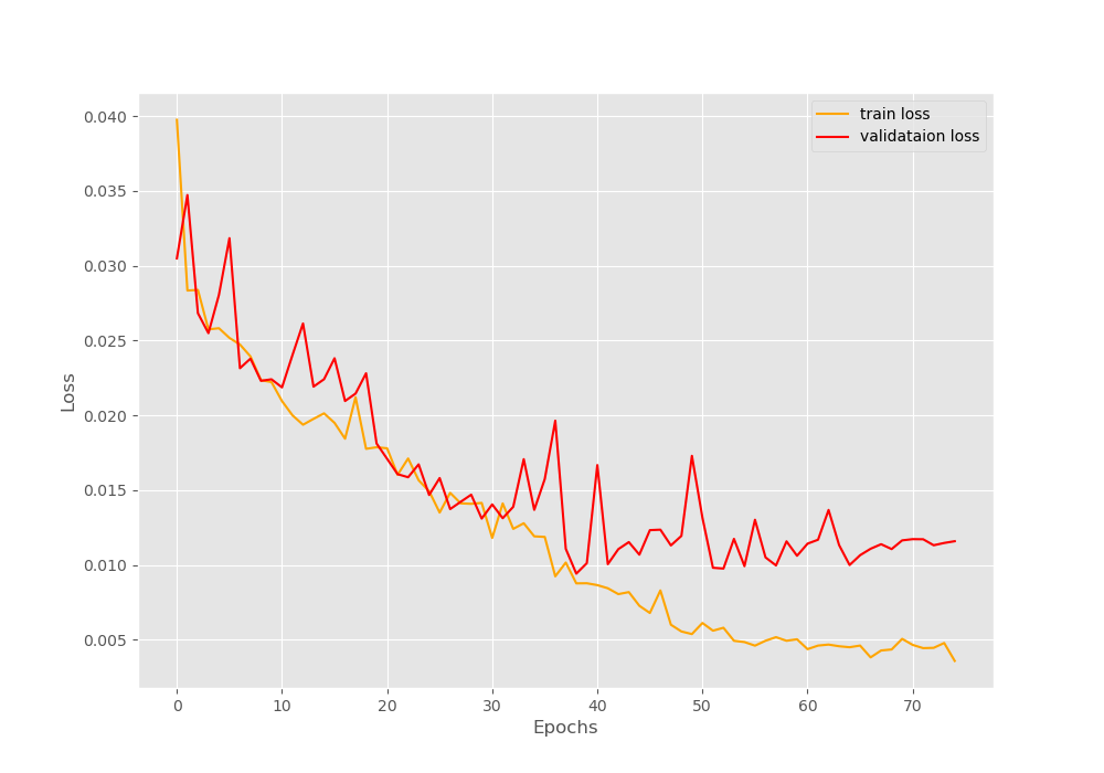
We can see that around the last 10 epochs, the validation loss is increasing bit. But the training loss is still decreasing. So, perhaps, using a lowered value factor in the learning rate scheduler would have helped. You can try that out and let me know in the comment section of your findings.

Moving on to the accuracy graph plot.

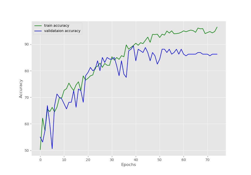
In the accuracy plot also, the validation accuracy is decreasing a bit after 60 epochs. Let’s hope that the model has learned the features well and can predict the video frames correctly while testing.

Testing the Trained Model for Action Recognition using Deep Learning on Real-Time Videos

We will write the test code for this tutorial now. All the code in this section will go into the test.py file.

I hope that you have obtained the video clips for testing using the links that I have provided in one of the previous sections.

Let’s start with importing the required modules and libraries.

'''
USAGE:
python test.py --model ../outputs/sports.pth --label-bin ../outputs/lb.pkl --input ../input/example_clips/chess.mp4 --output ../outputs/chess.mp4
'''

import torch
import numpy as np
import argparse
import joblib
import cv2
import torch.nn as nn
import torch.nn.functional as F
import time
import cnn_models
import albumentations

from torchvision.transforms import transforms   
from torch.utils.data import Dataset, DataLoader
from PIL import Image

You can see that we are importing both, OpenCV as well as the Python Imaging Library (PIL). This is because we will use OpenCV to read the video frames. And while training we have read the images using PIL. So, we will test our model by giving PIL format images to the model. The main reason for this is because of the difference between the RGB (Red, Green, Blue) and BGR (Blue, Green, Red) color formats of PIL and OpenCV.

Constructing the Argument Parser

We have four command line arguments while executing the test.py file.

# construct the argument parser
ap = argparse.ArgumentParser()
ap.add_argument('-m', '--model', required=True,
	help="path to trained serialized model")
ap.add_argument('-l', '--label-bin', required=True,
	help="path to  label binarizer")
ap.add_argument('-i', '--input', required=True,
	help='path to our input video')
ap.add_argument('-o', '--output', required=True, type=str,
	help='path to our output video')
args = vars(ap.parse_args())

• --model is the path to the saved model on the disk.
• --label-bin gives the path to the saved binarized labels files. We have saved this file while executing the prepare_data.py file.
• --input is the path to the input video clips that we will test our model on.
• --outputs is the path to save the output video clips after the video recognition takes place.

Load the Binarized Labels, Prepare the Model, and Define the Image Augmentations

We need to load the binarized labels to map the output tensors to the actual string labels (basketball or boxing or chess). We will also initialize the model here and load the saved weights to the model. Then we will define the image augmentations.

# load the trained model and label binarizer from disk
print('Loading model and label binarizer...')
lb = joblib.load(args['label_bin'])

model = cnn_models.CustomCNN().cuda()
print('Model Loaded...')

model.load_state_dict(torch.load(args['model']))
print('Loaded model state_dict...')

aug = albumentations.Compose([
    albumentations.Resize(224, 224),
    ])

For the augmentation, we will only be resizing the images into 224×224 dimensions.

Capturing the Video using OpenCV

We can easily read and capture video frames using cv2.VideoCapture(). We will also need the frame width and height that we will use while saving the output frames.

cap = cv2.VideoCapture(args['input'])

if (cap.isOpened() == False):
    print('Error while trying to read video. Plese check again...')

# get the frame width and height
frame_width = int(cap.get(3))
frame_height = int(cap.get(4))

# define codec and create VideoWriter object
out = cv2.VideoWriter(str(args['output']), cv2.VideoWriter_fourcc(*'mp4v'), 30, (frame_width,frame_height))

Also, we need to define the codec and specify the format for saving the video (line 11). We will save the video using MP4 format. All of the above functions are carried out by the following code block.

Reading the Frames and Carrying Out Predictions

We will read the video frame-by-frame until there are no more frames present. Then we will treat each frame as an image and carry out the predictions on each frame.

# read until end of video
while(cap.isOpened()):
    # capture each frame of the video
    ret, frame = cap.read()
    if ret == True:
        model.eval()
        with torch.no_grad():
            # conver to PIL RGB format before predictions
            pil_image = Image.fromarray(cv2.cvtColor(frame, cv2.COLOR_BGR2RGB))
            pil_image = aug(image=np.array(pil_image))['image']
            pil_image = np.transpose(pil_image, (2, 0, 1)).astype(np.float32)
            pil_image = torch.tensor(pil_image, dtype=torch.float).cuda()
            pil_image = pil_image.unsqueeze(0)
            
            outputs = model(pil_image)
            _, preds = torch.max(outputs.data, 1)
        
        cv2.putText(frame, lb.classes_[preds], (10, 30), cv2.FONT_HERSHEY_SIMPLEX, 0.9, (0, 200, 0), 2)
        cv2.imshow('image', frame)
        out.write(frame)

        # press `q` to exit
        if cv2.waitKey(27) & 0xFF == ord('q'):
            break

    else: 
        break

# release VideoCapture()
cap.release()

# close all frames and video windows
cv2.destroyAllWindows()

• We are capturing the frame at line 4. If there is a frame present, we enter the if block defined at line 5.
• Here also, we use the evaluation mode and the prediction takes place inside the with torch.no_grad() block (lines 6 and 7).
• Line 9 first reads the frame using the OpenCV and converts it into RGB format. Then it converts the image into the PIL image format.
• From lines 10 to 13:
  • We resize the image.
  • Then we transpose the dimensions to make the image channels-first.
  • At line 12, we convert the image into a torch tensor and transfer the image to GPU. Note that, if you have trained your model using CPU, then you need to use .cpu() instead of .cuda() at line 12.
  • At line 13, we unsqueeze the image to add an extra batch dimension.
• At line 15, we predict the output and at line 16, we get the prediction index.
• Line 18, puts the prediction string on the frame using the index position in the binarized labels file.
• Line 19, shows the frame on the screen and line 20 saves the frame to disk.
• Finally, we break out of the while loop, release the VideoCapture() object, and destroy all video capture windows.

Run the test.py File

First, let’s test the neural network model on the chess clip.

python test.py --model ../outputs/sports.pth --label-bin ../outputs/lb.pkl --input ../input/example_clips/chess.mp4 --output ../outputs/chess.mp4

The model is predicting the output as chess except for a single frame. In that single frame, the model is predicting the output class as basketball instead of chess. This is most probably because the video does not match the images very well that we trained our deep learning model on. In the train images, there were people surrounding chess boards and whole board was visible at all times.

Let’s try out another video.

python test.py --model ../outputs/sports.pth --label-bin ../outputs/lb.pkl --input ../input/example_clips/boxing1.mp4 --output ../outputs/boxing1.mp4

The model is predicting the boxing video perfectly. This means that the model has learned well on the boxing image data.

Finally, we will test the model on the basketball video.

python test.py --model ../outputs/sports.pth --label-bin ../outputs/lb.pkl --input ../input/example_clips/basketball.mp4 --output ../outputs/basketball.mp4

Interestingly, the model predicts the basketball class correctly as well. So, the model has not overfit and learned all the features of the data very well.

Moving Ahead from Here

If you wish to learn more about video predictions using deep learning, then you can look at the following resources.

• Retrieving actions in movies, Ivan Laptev and Patrick Perez.
• Learning realistic human actions from movies, Laptev et al.
• Finding Actors and Actions in Movies.
• An End-to-end 3D Convolutional Neural Network for Action Detection and Segmentation in Videos, Chen Chen.

Maybe after reading some papers, you will be ready to expand the project even further using larger datasets and including many more actions. You can also try extracting frames from videos to train the neural network. If you do expand the project, then do let me know in the comment section of your results. I will surely address your comment.

Summary and Conclusion

In this article, you learned how to carry action recognition in videos using deep learning and PyTorch.

• First, you trained a model on different sports images.
• Then you used the trained model to predict actions in real-time videos.

If you have any thoughts, doubts, or suggestions, then you can leave them in the comment section and I will surely address them.

You can contact me using the Contact section. You can also find me on LinkedIn, and Twitter.