Image Deblurring using Convolutional Neural Networks and Deep Learning

In this tutorial, you will learn how to carry out image deblurring using deep learning convolutional neural networks.

Deep learning for computer vision and images have shown incredible potential. This is the result of adapting the architectures of convolutional neural networks in deep learning to as many fields as possible. And the credit goes to Yann LeCun and many other deep learning scientists like him who made this a reality over the years.

There are many amazing results that we can achieve with deep convolutional neural networks. Starting from image classification, recognition, localization, object detection, and many more. And image deblurring is one such amazing feat that we can achieve with deep learning and convolutional neural networks.

What Will You Learn in This Tutorial?

• A brief on deblurring of images using deep learning.
• The SRCNN architecture that we will use for image deblurring.
• Coding our way through deblurring of images using deep learning and convolutional neural networks.

Image Deblurring and Image Super-Resolution using Deep Learning

There are many research works trying to tackle the problem of image deblurring and image super-resolution using deep learning.

Basically, the following is the concept behind image deblurring using deep learning:

• We have an image dataset that is the original high-resolution images.
• We will add some type of noise, or blur them, or reduce their resolution to obtain a new image dataset.
• Then we will apply a deep learning architecture trying to get back the high-resolution images from the noisy, or blurred, or low-resolution images.

In theory, it sounds simple. But in practice, trying to get the desired results is more complicated. Many times, the final results are not what we expect. Maybe the deep learning architecture is at fault or maybe the approach to the problem is not optimal. That being said, there is much successful research around this field as well.

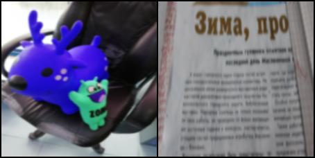
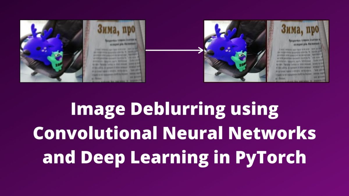
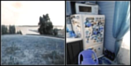
Figures 1 and 2 show an example of what to expect in image deblurring. Figure 1 shows an image to which Gaussian blurring has been added. Then this image goes through a deep learning architecture which gives us the result as Figure 2.

We will try to achieve something similar to the above results in this tutorial

Some Successful Results Around Image Deblurring and Super-Resolution using Deep Learning

What we will discuss here is in no way an exhaustive list of all the research work that has been going around. These are only the research papers that I was able to go through for writing this tutorial. And we will try to follow the convolutional neural network architecture from one of the papers.

Single Image Super-Resolution

Here, we will discuss the paper named Image super-resolution as sparse representation of raw image patches by Jianchao Yang, John Wright, Thomas S. Huang, and Yi Ma.

In this paper, they try to address the problem of obtaining a high-resolution image from a single resolution image.

The following is a quote from the abstract section of the paper.

This paper addresses the problem of generating a super- resolution (SR) image from a single low-resolution input image. We approach this problem from the perspective of compressed sensing.

Image super-resolution as sparse representation of raw image patches by Jianchao Yang, John Wright, Thomas S. Huang, and Yi Ma.

Single image super-resolution using deep learning is a very active field of research. You can try out and apply some research papers to replicate the results. This will give you a very firm understanding of the concepts.

Image Deblurring using Convolutional Neural Networks

One of the recent papers in image deblurring and super-resolution using convolutional neural networks is by Fatma Albluwi, Vladimir A. Krylov & Rozenn Dahyot.

Their paper Image Deblurring and Super-Resolution Using Deep Convolutional Neural Networks is one of the most recent works in the field (2018).

The related problem of super-resolution from blurred or corrupted low-resolution images has however received much less attention. In this work, we propose a new deep learning approach that simultaneously addresses deblurring and super-resolution from blurred low-resolution images.

Image Deblurring and Super-Resolution Using Deep Convolutional Neural Networks.

In this paper, they try to address the problem of image deblurring and image super-resolution together. You should surely give this paper a read to get a deeper understanding of the approach used. Also, they try to follow on the work of Chao Dong, Chen Change Loy, Kaiming He, Xiaoou Tang who proposed the state-of-the-art SRCNN architecture for image super-resolution.

Image Super-Resolution Using Deep Convolutional Networks

In 2014, Chao Dong, Chen Change Loy, Kaiming He, Xiaoou Tang, released a paper titled Learning a Deep Convolutional Network for Image Super-Resolution.

In this paper, they introduced a new state-of-the-art convolutional neural network architecture for image super-resolution. They termed it as the SRCNN (Super-Resolution Convolutional Neural Network).

Quoting the first few lines of the abstract from their paper will give us a better idea of what the aim of the research was.

We propose a deep learning method for single image super-resolution (SR). Our method directly learns an end-to-end mapping between the low/high-resolution images. The mapping is represented as a deep convolutional neural network (CNN) that takes the low-resolution image as the input and outputs the high-resolution one.

Learning a Deep Convolutional Network for Image Super-Resolution, Chao Dong, Chen Change Loy, Kaiming He, Xiaoou Tang.

So, the authors built a convolutional neural network architecture that takes in a low-resolution image and outputs a high-resolution image. Most of such works were considered to be possible with autoencoders, but it is possible with convolutional neural networks as well.

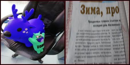
The following image shows some of the results from the SRCNN paper.

In Figure 3, you can see the comparison between three methods. The bicubic, SC (sparse coding), and SRCNN. And you can see that SRCNN has the highest PSNR (Peak Signal to Noise Ratio). Also, the super-resolution of the butterfly wing beside the graph has the best results in the case of SRCNN.

Let’s take a better look at the SRCNN architecture.

The SRCNN Architecture

We will go over the SRCNN architecture briefly in this section.

The best part of the SRCNN architecture is that it is really simple. If you are into deep learning, then you will not have any difficulties in understanding the architecure.

The SRCNN architecture has a total of three convolutional layers. The following two figures summarize the architecture of SRCNN.

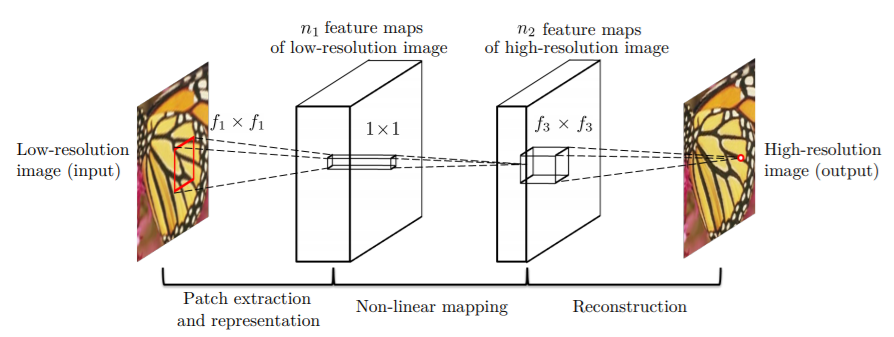
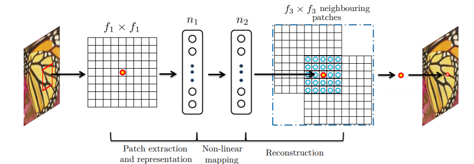
Let’s summarize Figures 4 and 5. First, we have a convolution operation where the weight matrix is of shape \(c\) x \(f_1\) x \(f_1\) x \(n_1\). Here, \(c\) is the number of channels, \(f_1\) is the number of kernels, and \(n_1\) is the number of filters or neurons.

For the second convolution operation, the weight matrix \(W_2\) is of size \(n_1\) x \(1\) x \(1\) x \(n_2\). Here, the kernels are of 1×1 size.

Similarly, the third convolution operation involves a weight matrix \(W_3\) of size \(n_2\) x \(f_3\) x \(f_3\) x \( c \). Here, the \(c\) is again the number of channels.

Among all those three convolution operations, ReLU (Rectified Linear Units) activations are applied to the first two convolution operations.

We will not go into the further details of the architecture, as it is out of scope of this tutorial. Instead, we will focus on practical coding very shortly. But do try to give the paper a read, this will make many things clearer to you.

The Implementation of SRCNN in Coding

This GitHub repository by YapengTian shows the implementation of SRCNN using Keras. The following are practical implementation from the repository:

• \(n_1\) = 64.
• \(n_2\) = 32
• \(n_3\) = 1
• \(f_1\) = 9
• \(f_2\) = 1
• \(f_3\) = 5

The code in the repository used 33×33 dimensional images.

Implementation in this Tutorial

There are some major changes of what we are going to do in this tutorial.

• Instead of the dataset used in the papers, we will use a Kaggle dataset.
• We will not carry out super-resolution, instead, we will try to deblur the Gaussian blurred images.
• We will use PyTorch deep learning library in this tutorial.
• The Keras implementation used 33×33 dimensional images, but we will use 224×224 dimensional images.

The architecture of the neural network will remain same as the original.

Now, let’s get to the implementation part.

The Dataset

We will use the Blur Dataset from Kaggle. This dataset contains a total of 1050 images. There are three categories, sharp images, defocused blur image, and motion-blur images. So, each of the directories contains 350 images.

An image in the dataset contains triplets of sharp image, defocused blur image and motion-blurred image. So, the same image has three instances and in its respective directory.

But we will not be using the defocused blur images or motion-blurred images for deblurring in this tutorial. Instead, we will add Gaussian blurring to the sharp images and deblur those images. The reason for this is that motion-blurred and the defocused blur images have a pixel translation in the dataset. The blurred images in the dataset have a bit of shifting while trying to replicate the blurring when taking the photos.

Deblurring images with pixel translation to the original image requires a different approach than what we are trying to achieve in this tutorial. I hope that I will be able to address it in one of the future tutorials.

Download the dataset and explore it a bit.

The Directory Structure

The following is the directory structure for this tutorial.

├───input
│   ├───defocused_blurred
│   ├───gaussian_blurred
│   ├───motion_blurred
│   └───sharp
├───outputs
│   └───saved_images
└───src
│   add_gaussian_blur.py
│   deblur.py

• input folder contains the data that we will use. After extracting the downloaded dataset, you will have three folder, sharp, defocused_blurred, and motion_blurred. As discussed above, we will add Gaussian blurring to the sharp images. These images will reside in the gaussian_blurred folder. We will not use the defocused_blurred or the motion_blurred images.
• outputs folder will contain the output files that we will get after training. It also has a saved_images folder that will contain the deblurred images that we will get during validation.
• src folder contains two python file. The add_gaussian_blur.py file will contain the code to add Gaussian blurring to the sharp images. The deblur.py file will contain the code to deblur the blurred images.

Go, ahead and create the directory structure and familiarize yourself with the dataset a bit. Next we will move onto coding.

Adding Gaussian Blurring to the Sharp Images

In this section, we will add Gaussian blurring to the sharp images. All the code in this section will go into the add_gaussian_blur.py file.

The code is fairly simple. We will use the OpenCV library to read the images, add Gaussian blurring, and write the blurred images back to disk.

If you need to learn more about the blurring of images, then you can check out this tutorial. I hope that you will learn a lot.

Let’s import the libraries and modules that we need.

import cv2
import os
import numpy as np

from tqdm import tqdm

os.makedirs('../input/gaussian_blurred', exist_ok=True)

src_dir = '../input/sharp'
images = os.listdir(src_dir)
dst_dir = '../input/gaussian_blurred'

In the above code block, first we import OpenCV, NumPy, os, and tqdm. These are the modules that we need.

• Then we make the gaussian_blurred folder inside the input folder at line 7.
• At line 9, we get a hold on the sharp images directory and at line 10, we get all the sharp image paths as a list.
• Line 11 defines the destination directory where the blurred images will be saved.

Adding Gaussian Blurring

Adding Gaussian blurring to the images is just one line of code using OpenCV.

We will loop over the total number of images, read the images, and add Gaussian blurring using cv2.GaussianBlur() function. Finally, we will write the blurred images back to disk.

The following block of code does that for us.

for i, img in tqdm(enumerate(images), total=len(images)):
    img = cv2.imread(f"{src_dir}/{images[i]}", cv2.IMREAD_COLOR)
    # add gaussian blurring
    blur = cv2.GaussianBlur(img, (31, 31), 0)
    cv2.imwrite(f"{dst_dir}/{images[i]}", blur)

print('DONE')

We are adding Gaussian blurring to the image with a kernel size of 31×31.

You can execute the code by typing the following command in the terminal while being within the src folder.

python add_gaussian_blur.py

It will take just a few seconds to execute.

Now, let’s take a loot at how the Gaussian blurred images look like when compared with the sharp images.

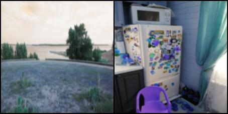
Figure 6 shows the original sharp image from the sharp folder. And Figure 7 shows the Gaussian blurred images that we will deblur using deep learning. You can see that the second image is a lot blurrier than the sharp image. This is going to be a lot interesting to see what final results we get after deblurring.

Writing the Code to Deblur the Gaussian Blurred Images

From here on, we will write the code to deblur the Gaussian blurred images. The code from here on will go into the deblur.py file.

Importing the Required Modules and Libraries

Let’s start with importing the modules and libraries that we will need to carry on further.

import numpy as np
import os
import matplotlib.pyplot as plt
import glob
import cv2
import torch
import torchvision
import torch.nn as nn
import torch.nn.functional as F
import torch.optim as optim
import time
import argparse

from tqdm import tqdm
from torch.utils.data import Dataset, DataLoader
from torchvision.transforms import transforms
from torchvision.utils import save_image
from sklearn.model_selection import train_test_split

The above code block imports all the modules and libraries that we need to deblur the images in this tutorial. Familiarity with PyTorch will help you a lot to carry on further.

One of the important modules that we are importing is the save_image module from torchvision. The save_image module helps us to easily save the images in batches as they are used in the DataLoader.

Defining Argument Parser and Helper Function for Saving Image

Let’s define the argument parser for the number of epochs. We will also define the helper function to save the deblurred images during validation.

# constructing the argument parser
parser = argparse.ArgumentParser()
parser.add_argument('-e', '--epochs', type=int, default=40, 
            help='number of epochs to train the model for')
args = vars(parser.parse_args())

def save_decoded_image(img, name):
    img = img.view(img.size(0), 3, 224, 224)
    save_image(img, name)

• The default number of epochs is 40. --epochs is the only command line argument that we will give while executing the program.
• Starting from line 7, we define the save_decoded_image() function. We will call this image while validating the model to save the deblurred images.

Now, we will create the saved_images folder inside the outputs folder.

# helper functions
image_dir = '../outputs/saved_images'
os.makedirs(image_dir, exist_ok=True)

device = 'cuda:0' if torch.cuda.is_available() else 'cpu'
print(device)

batch_size = 2

• In the above code block, we are also selecting the computation device. It is better if you have a GPU in your system for running the program.
• We are defining a batch size of 2 as well.

Define Train-Test Split and the Image Transforms

In this section, we will define the training and validation split and define the image transforms as well.

Let’s start with getting hold of all the image file paths.

gauss_blur = os.listdir('../input/gaussian_blurred')
gauss_blur.sort()
sharp = os.listdir('../input/sharp')
sharp.sort()

x_blur = []
for i in range(len(gauss_blur)):
    x_blur.append(gauss_blur[i])

y_sharp = []
for i in range(len(sharp)):
    y_sharp.append(sharp[i])

• gauss_blur and sharp are two lists containing the image file paths to the blurred and sharp images respectively. We are also sorting the list so that the corresponding blurred and sharp image file paths align with each other.
• Then we define two more lists, x_blur and y_sharp which contain the Gaussian blurred and sharp image paths respectively. x_blur will act as the training data and y_blur will act as the label. So, while training we compare the blurred image outputs with the sharp image. We will try to make the blurred images as similar to the sharp images as possible.

The following block of code defines the training and validation split. We will use 75% of the data for training and 25% of the data for validation.

(x_train, x_val, y_train, y_val) = train_test_split(x_blur, y_sharp, test_size=0.25)

print(f"Train data instances: {len(x_train)}")
print(f"Validation data instances: {len(x_val)}")

Next, let’s define the image transforms.

# define transforms
transform = transforms.Compose([
    transforms.ToPILImage(),
    transforms.Resize((224, 224)),
    transforms.ToTensor(),
])

• First, we are converting the image to PIL image format.
• Then we are resizing the image to 224×224 dimensions.
• Finally, we are converting the image to torch tensors.

Note that we are not applying any other transforms like rotating or shifting. This is so that the blurred images and sharp images have the same pixel translation without any misalignment.

The Dataset and DataLoader

Here, we will define the custom dataset using the PyTorch Dataset class. We will call this module DeblurDataset().

The following block of code defines the DeblurDataset() module.

class DeblurDataset(Dataset):
    def __init__(self, blur_paths, sharp_paths=None, transforms=None):
        self.X = blur_paths
        self.y = sharp_paths
        self.transforms = transforms
         
    def __len__(self):
        return (len(self.X))
    
    def __getitem__(self, i):
        blur_image = cv2.imread(f"../input/gaussian_blurred/{self.X[i]}")
        
        if self.transforms:
            blur_image = self.transforms(blur_image)
            
        if self.y is not None:
            sharp_image = cv2.imread(f"../input/sharp/{self.y[i]}")
            sharp_image = self.transforms(sharp_image)
            return (blur_image, sharp_image)
        else:
            return blur_image

• In the __init__() function (line 2), we initialize the blurred images paths, sharp images paths, and the image transforms.
• Starting from line 10, we have the __getitem__() function.
  • First, we read the blurred image from the blurred image paths. Then we apply the transforms to the images.
  • At line 17, we read the sharp images, which will act as the labels while training and validating. We are applying the same transform to the sharp images as well.

Next, we will define the train data, validation data, train loader, and validation loader. We will use a batch size of 2 as defined above. Also, we will shuffle the training data only and not the validation data.

train_data = DeblurDataset(x_train, y_train, transform)
val_data = DeblurDataset(x_val, y_val, transform)
 
trainloader = DataLoader(train_data, batch_size=batch_size, shuffle=True)
valloader = DataLoader(val_data, batch_size=batch_size, shuffle=False)

We are all set with our dataset. Next, we will define our convolutioal neural network architecture.

The Convolutional Neural Network Architecture

Our convolutional neural network architecture will be similar to SRCNN architecture. But we will call the neural network architecture as DeblurCNN().

class DeblurCNN(nn.Module):
    def __init__(self):
        super(DeblurCNN, self).__init__()

        self.conv1 = nn.Conv2d(3, 64, kernel_size=9, padding=2)
        self.conv2 = nn.Conv2d(64, 32, kernel_size=1, padding=2)
        self.conv3 = nn.Conv2d(32, 3, kernel_size=5, padding=2)

    def forward(self, x):
        x = F.relu(self.conv1(x))
        x = F.relu(self.conv2(x))
        x = self.conv3(x)

        return x

model = DeblurCNN().to(device)
print(model)

You can see that our DeblurCNN() architecture is very similar to the SRCNN architecture. The only notable difference is the application of zero-padding. Applying the zero-padding to each convolutional layer ensures that the output have the same dimensions as inputs for each layer.

We need to define the optimizer and the loss function as well. Along with that, we will also define a learning rate scheduler. Let’s take a look at the code.

# the loss function
criterion = nn.MSELoss()
# the optimizer
optimizer = optim.Adam(model.parameters(), lr=0.001)
scheduler = torch.optim.lr_scheduler.ReduceLROnPlateau( 
        optimizer,
        mode='min',
        patience=5,
        factor=0.5,
        verbose=True
    )

• We are using the MSE (Mean Square Error Loss) as we will be comparing the pixels of blurred images and sharp images.
• The optimizer is Adam with a learning rate of 0.001.
• We are also defining a ReduceLROnPlateau() learning rate scheduler. The patience is 5 and factor is 5. So, if the loss value does not improve for 5 epochs, the new learning rate will be old_learning_rate * 0.5.

The Training Function

The training function is going to be very simple. We will call this function as fit(). The following code block defines the training function.

def fit(model, dataloader, epoch):
    model.train()
    running_loss = 0.0
    for i, data in tqdm(enumerate(dataloader), total=int(len(train_data)/dataloader.batch_size)):
        blur_image = data[0]
        sharp_image = data[1]
        blur_image = blur_image.to(device)
        sharp_image = sharp_image.to(device)
        optimizer.zero_grad()
        outputs = model(blur_image)
        loss = criterion(outputs, sharp_image)
        # backpropagation
        loss.backward()
        # update the parameters
        optimizer.step()
        running_loss += loss.item()
    
    train_loss = running_loss/len(dataloader.dataset)
    print(f"Train Loss: {train_loss:.5f}")
    
    return train_loss

• We are only keeping track of the loss values while training. running_loss keeps track of the batch-wise loss.
• Take a look at the loss at line 11. We are calculating the loss for the outputs and the sharp_image. This is because we want to make the blurry images as similar to the sharp images as possible.
• At line 18, we are calculating the loss for each epoch (train_loss). We are returning the train_loss value at line 21.

The Validation Function

We will call the validation function as validate().

def validate(model, dataloader, epoch):
    model.eval()
    running_loss = 0.0
    with torch.no_grad():
        for i, data in tqdm(enumerate(dataloader), total=int(len(val_data)/dataloader.batch_size)):
            blur_image = data[0]
            sharp_image = data[1]
            blur_image = blur_image.to(device)
            sharp_image = sharp_image.to(device)
            outputs = model(blur_image)
            loss = criterion(outputs, sharp_image)
            running_loss += loss.item()

            if epoch == 0 and i == int((len(val_data)/dataloader.batch_size)-1):
                save_decoded_image(sharp_image.cpu().data, name=f"../outputs/saved_images/sharp{epoch}.jpg")
                save_decoded_image(blur_image.cpu().data, name=f"../outputs/saved_images/blur{epoch}.jpg")

            if i == int((len(val_data)/dataloader.batch_size)-1):
                save_decoded_image(outputs.cpu().data, name=f"../outputs/saved_images/val_deblurred{epoch}.jpg")

        val_loss = running_loss/len(dataloader.dataset)
        print(f"Val Loss: {val_loss:.5f}")
        
        return val_loss

The whole validation takes place within the with torch.no_grad() block. This ensures that the gradients do not get calculated during validation.

• We are keeping track of the validation loss values. But we do no need to backpropagate the gradients or update the parameters.
• Starting from line 14 till 16, we saving one instance of the sharp image and the blurred image from the last batch. This will help us compare the blurred, sharp and deblurred images.
• Then at line 18 and 19, we saving the last deblurred image from the last batch. This takes place every epoch. So, by the end of the training we will have 40 deblurred images (one image per epoch) in the saved_images folder.

Executing the Training and Validation Function

We will execute the training and validation functions for the number of epochs specified in the command line.

train_loss  = []
val_loss = []
start = time.time()
for epoch in range(args['epochs']):
    print(f"Epoch {epoch+1} of {args['epochs']}")
    train_epoch_loss = fit(model, trainloader, epoch)
    val_epoch_loss = validate(model, valloader, epoch)
    train_loss.append(train_epoch_loss)
    val_loss.append(val_epoch_loss)
    scheduler.step(val_epoch_loss)
end = time.time()

print(f"Took {((end-start)/60):.3f} minutes to train")

We are storing the train and validation loss values of each epoch in the train_loss and val_loss lists respectively. At line 10, we are applying the learning rate scheduler as well.

Finally, we need to save the loss plot to the disks. This will later help us to analyze the performance of the model. We will also save the trained model to disk.

# loss plots
plt.figure(figsize=(10, 7))
plt.plot(train_loss, color='orange', label='train loss')
plt.plot(val_loss, color='red', label='validataion loss')
plt.xlabel('Epochs')
plt.ylabel('Loss')
plt.legend()
plt.savefig('../outputs/loss.png')
plt.show()

# save the model to disk
print('Saving model...')
torch.save(model.state_dict(), '../outputs/model.pth')

Run the deblur.py File and Analyze the Results

Now we get to run the deblur.py file. We will train the neural network model for 40 epochs.

python deblur.py --epochs 40

The following is the truncated output after running the file.

cuda:0
Train data instances: 262
Validation data instances: 88
DeblurCNN(
(conv1): Conv2d(3, 64, kernel_size=(9, 9), stride=(1, 1), padding=(2, 2))
(conv2): Conv2d(64, 32, kernel_size=(1, 1), stride=(1, 1), padding=(2, 2))
(conv3): Conv2d(32, 3, kernel_size=(5, 5), stride=(1, 1), padding=(2, 2))
)
Epoch 1 of 40
100%|████████████████████████████████████████████████████████████████| 131/131 [01:00<00:00,  2.15it/s]
Train Loss: 0.00728
100%|██████████████████████████████████████████████████████████████████| 44/44 [00:19<00:00,  2.23it/s]
Val Loss: 0.00345
...
Epoch 40 of 40
100%|████████████████████████████████████████████████████████████████| 131/131 [00:45<00:00,  2.85it/s]
Train Loss: 0.00019
100%|██████████████████████████████████████████████████████████████████| 44/44 [00:14<00:00,  3.06it/s]
Val Loss: 0.00018
Took 42.719 minutes to train
Saving model...

Let’s take a look at the graphical plot of the loss values that is saved to the disk.

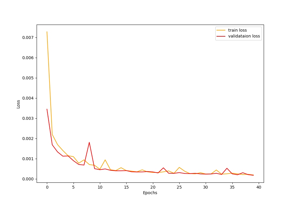
In Figure 8, we can see that the loss decreases rapidly until 10 epochs, and then it starts to decrease slowly. But still, it keeps on improving till 40 epochs. By the end of 40 epochs, we are getting a train loss of 0.00019 and a validation loss of 0.00018. From the values, it seems the model has learned well. But was the neural network model able to deblur the blurred images?

Analyzing the Saved Images

In this section, we will analyze the saved images in the outputs folder. Let’s see whether our model was able to deblur the images or not.

In Figure 9 you can see that the image is much blurrier than the original sharp image. In fact, it is even blurrier than the Gaussian blurred image that we have seen above.

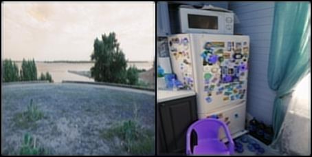
Figure 10 shows the output after 10 epochs. We can see that the neural network model is able to deblur the image to some extent. Let’s hope that it has even better performance in the later epochs as well.

Figure 11 shows the deblurred image after 40 epochs, that is, the final epoch. We can see that the convolutional neural network model is almost able to deblur the image. This is really interesting. We are getting such good results from such a simple convolutional neural network.

What Can You Improve Upon Further?

There are some things that you can improve upon to make it a full-fledged deep learning project.

• First of all, get your hands on some research papers on deblurring and super-resolution using deep learning. You will gain a lot of ideas.
• In this small project, the blurred and the original images did not have any pixel translation. But the other two folders, motion_blurred and defocused_blurred have images that are a little bit shifted in comparison to the original images.
• Now, deblurring images that have pixel translation is trickier and more complex than the approach that we have discussed here. But you can try out the project and improve upon it even further.
• Trying out single image super-resolution. In this case, you use only one image for deblurring and image super-resolution. Challenging, but you will learn a lot.
• Finally, read and try out the codes online, on GitHub, other platforms. See other people’s approaches and try improving your own approach.

Summary and Conclusion

In this tutorial you learned how to deblur Gaussian blurred images using deep learning and convolutional neural networks. We discussed three research papers in brief. Along with that, you had a hands-on coding experience on how to deblur the blurred images using deep learning and PyTorch. I hope that you learned a lot in this tutorial.

You can leave your thoughts and doubts in the comment section, and I will surely address them.

You can contact me using the Contact section. You can also find me on LinkedIn, and Twitter.