American Sign Language Recognition using Deep Learning

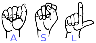
In this article, you will use deep learning and convolutional neural networks to recognize American Sign Language (ASL) alphabets. Specifically, you will learn to carry out American Sign Language recognition using deep learning and neural networks.

Why this Project?

The users of American Sign Language range somewhere between 250,000 to 500,000 persons. But most of the communication happens among the persons suffering from deafness and those who have learned American Sign Language. If someone who is not proficient wants to communicate, then he or she needs someone who has learned American Sign Language. There are experts in sign language who act as moderators between the person who is verbally speaking and the disabled person who is using sign language.

In this tutorial, we will try to build a deep learning model to alleviate the problem a bit. We will use deep learning and convolutional neural networks to build a model for American Sign Language recognition with decent enough accuracy.

Note: I am not claiming that this model will be 100% accurate. But this can be a starting point to build it into a much larger project from here on. This small project can be used as a stepping stone to build a system that can further be used to recognize words and sentences.

Deep Learning for Computer Vision has shown real potential in the last few years. It has solved many real-world problems which seemed impossible previously. And deep learning for computer vision will continue to do so in the future as well. This is just another small project to show how much deep learning is useful to solve real-world problems.

What Will You Learn in This Project?

So, what are the things that you will learn after completing this tutorial? The following list will give you a good idea.

• Using deep learning and neural networks to build an American Sign Language Recognizer for images.
• Using deep learning to recognize American Sign Language in webcam video feed in real-time.
• Managing large image datasets and using a subset of images to train your deep neural network.

Some important libraries and packages you need before moving further:

• I recommend that you install PyTorch deep learning library. The code in this tutorial uses PyTorch and for starting out you can refer to this series.
• Another package that I highly recommend is the imutils package which helps a lot when handling image file paths. You can install it from here.
• Also, you need the Albumentations library to carry out image augmentations in this tutorial. This is a really good library with really good documentation and examples.

The Dataset and Directory Structure

We will the ASL Alphabet dataset from Kaggle. This is a very large dataset containing 87000 images. All the images are 200×200 in dimension.

You can go ahead and download the dataset. It will download as a .zip file.

In this dataset, there are 29 classes in total. 26 of these classes are letters from A-Z. Then there are three more classes that correspond to  SPACE, DELETE, and NOTHING. These three more classes will become really essential if you will want to take on the task to expand the project into something much larger. So, there are 3000 images from each class.

But we will not be using all the images to train our convolutional neural network for American Sign Language recognition. It will take much more time and resources. In fact, we will just use a subset of the images as a starting point. We will get to more about this while preparing the dataset.

All of the images are inside their corresponding class folders.

Here are a few images from the training dataset.

The Directory Structure

The following is the directory structure for this tutorial.

├───input
│   ├───asl_alphabet_test
│   │   └───asl_alphabet_test
│   ├───asl_alphabet_train
│   │   └───asl_alphabet_train
│   │       ├───A
│   │       ├───B
│   │       ...
│   └───preprocessed_image
│       ├───A
│       ├───B
│       ├───C
│       ...
|   data.csv
├───outputs
└───src
│   cam_test.py
│   cnn_models.py
│   create_csv.py
│   preprocess_image.py
│   test.py
│   train.py    

There are three main folder there, input, outputs, and src. Let’s go through each one of them.

• After extracting the downloaded zip file, you will get the folders asl_alphabet_train, and asl_alphabet_test. Those are inside the input folder first. They contain sub-folders by the same name again.
  • The asl_alphabet_train subfolder contains different class folders and images (A-Z, space, delete, nothing).
  • The asl_alphabet_test sub-folder contains some images that we can use for testing.
  • Then we have the preprocessed_image folder containing the class folders and the images again. These are the subset of images that we will use for training. We will get to the creation of these preprocessed images while writing the code. But we will not go into the detailed explanation of the code in this tutorial.
  • We also have a data.csv file. This file contains the image paths and the labels corresponding to those paths. We will also create this file while coding.
• The outputs folder will contain all the training and testing outputs. This includes the trained models, loss, and accuracy plots as well.
• The src folder contains:
  • train.py: We will write the training code inside this file.
  • test.py: We will write the code to test images inside this file.
  • cnn_models.py: This file will contain our convolutional neural network architecture.
  • cam_test.py: We will use this file to test our trained deep learning model on real-time webcam feed for recognizing the alphabets.
  • preprocess_image.py: We will use this file to create the subset of images (preprocessed_image) folder.
  • create_csv.py: This file will contain the code to create the data.csv file.

Take some time to explore all the files and folders.

American Sign Language Recognition using Deep Learning

Beginning from this section, we will get into writing the Python code for this tutorial. The following are the steps we will follow.

• Creating the preprocessed images.
• Creating the data.csv file.
• Writing the training code inside the train.py file.
• Writing our neural network architecture inside cnn_models.py file.
• Preparing the test code.
• Then we will write the code for detecting the sign language letters inside cam_test.py file for real-time webcam feed.

So, the above are the six major steps we will go through in this tutorial. I hope that after this, you will have a better idea of how to set up a small scale/medium scale project for deep learning. You will learn about using a subset of images, and not the whole 87000 images. So, I hope that’s something new you learn as well. Let’s start.

Preprocessing a Subset of Images

In this section, we will write the code to preprocess a subset of images out of the total 87000 images. We will use these many images for training. Later on, you can also try out training your deep neural network on the whole set of images as well.

There are 3000 images from each class. But we will only use 1200 images from each class. So, that will be a total of 34800 images.

Let’s get to the coding part. From here on, unless I have stated otherwise, all the code will go into the preprocess_image.py file.

Imports and Building the Argument Parser

'''
USAGE:
python preprocess_image.py --num-images 1200
'''

import os
import cv2
import random
import numpy as np
import argparse

from tqdm import tqdm

parser = argparse.ArgumentParser()
parser.add_argument('-n', '--num-images', default=1200, type=int,
    help='number of images to preprocess for each category')
args = vars(parser.parse_args())

print(f"Preprocessing {args['num_images']} from each category...")

The modules that we import are very generic to python and machine learning.

• We will use cv2 to read and preprocess images.
• argparse for parsing command line arguments.
• imutils for getting proper image paths.
• From lines 15 to 18, we build the argument parser and parse the arguments. There is only one command-line argument. That is --num-images which specifies the number of images that we want to preprocess from each category.

Get All the Directory Paths

We need all the directory paths to all the classes. The following code block does that for us.

# get all the directory paths
dir_paths = os.listdir('../input/asl_alphabet_train/asl_alphabet_train')
dir_paths.sort()

root_path = '../input/asl_alphabet_train/asl_alphabet_train'

• dir_paths contains all the class folder paths, from A to Z, along with del, nothing, and space.
• We sort all the dir_paths as well.
• Finally at line 6, we define the root_path to the images.

The usage of all the above paths will become very clear in the next section of coding.

Preprocessing the Images and Saving them to Disk

Let’s write the code first. This will make things much clearer.

# get --num-images images from each category
for idx, dir_path  in tqdm(enumerate(dir_paths), total=len(dir_paths)):
    all_images = os.listdir(f"{root_path}/{dir_path}")
    os.makedirs(f"../input/preprocessed_image/{dir_path}", exist_ok=True)
    for i in range(args['num_images']): # how many images to preprocess for each category
        # generate a random id between 0 and 2999
        rand_id = (random.randint(0, 2999))
        image = cv2.imread(f"{root_path}/{dir_path}/{all_images[rand_id]}")
        image = cv2.resize(image, (224, 224))

        cv2.imwrite(f"../input/preprocessed_image/{dir_path}/{dir_path}{i}.jpg", image)

print('DONE')

Getting to the explanation of the above code:

• Starting from line 2, we loop over all the dir_paths.
• At line 3, we get hold of all the images in that respective class directory. So, if the directory is A, then all_images will contain all the images in the A folder.
• At line 4, we make the preprocessed_image folder and inside that the class folder which we are currently looping over.
• From line 5, we have another for loop which will go on for the --num-images number of times.
• At line 7, we generate a random number so that we can randomly pick images.
• Then from lines 8 to 11, we read, resize and save the resized images to disk.

We are just resizing the images. In deep learning for computer vision, often no further preprocessing of images is required besides resizing. That’s why we can build end-to-end systems using deep learning.

Now execute the preprocess_image.py file while within the src folder in the terminal.

python preprocess_image.py --num-images 1200

Your output should be similar to the following.

Preprocessing 1200 from each category...
...
DONE

Creating the data.csv File

In this section, we will create the data.csv file.

The data.csv file maps the image paths to the target classes. So, it will contain two columns. One is the image_path column which will contain all the image paths. The second column is the target column which will be a number between 0 and 28 that indicates the class of the image.

The code in this section will go into create_csv.py file.

We will not go into the explanation of the code in this section. So, please do take some time to review this code and what it’s doing. The code is not complex. It is just a few lines of python code of writing data into a Data Frame and saving is as a CSV file.

The Code for create_csv.py File

'''
USAGE:
python create_csv.py
'''

import pandas as pd
import numpy as np
import os
import joblib

from sklearn.preprocessing import LabelBinarizer
from tqdm import tqdm
from imutils import paths

# get all the image paths
image_paths = list(paths.list_images('../input/preprocessed_image'))

# create a DataFrame 
data = pd.DataFrame()

labels = []
for i, image_path in tqdm(enumerate(image_paths), total=len(image_paths)):
    label = image_path.split(os.path.sep)[-2]
    # save the relative path for mapping image to target
    data.loc[i, 'image_path'] = image_path

    labels.append(label)

labels = np.array(labels)
# one hot encode the labels
lb = LabelBinarizer()
labels = lb.fit_transform(labels)

print(f"The first one hot encoded labels: {labels[0]}")
print(f"Mapping the first one hot encoded label to its category: {lb.classes_[0]}")
print(f"Total instances: {len(labels)}")

for i in range(len(labels)):
    index = np.argmax(labels[i])
    data.loc[i, 'target'] = int(index)

# shuffle the dataset
data = data.sample(frac=1).reset_index(drop=True)

# save as CSV file
data.to_csv('../input/data.csv', index=False)

# pickle the binarized labels
print('Saving the binarized labels as pickled file')
joblib.dump(lb, '../outputs/lb.pkl')

print(data.head(5))

Execute the python file.

python create_csv.py

You should get the following output.

...
The first one hot encoded labels: [1 0 0 0 0 0 0 0 0 0 0 0 0 0 0 0 0 0 0 0 0 0 0 0 0 0 0 0 0]
Mapping the first one hot encoded label to its category: A
Total instances: 34800
Saving the binarized labels as pickled file
                               image_path  target
0  ../input/preprocessed_image\L\L973.jpg    11.0
1   ../input/preprocessed_image\B\B41.jpg     1.0
2  ../input/preprocessed_image\L\L435.jpg    11.0
3  ../input/preprocessed_image\M\M483.jpg    12.0
4  ../input/preprocessed_image\Y\Y370.jpg    24.0

Note that executing this file also creates a lb.pkl file inside the outputs folder. This file contains the binarized labels. It also contains an attribute called as classes_. And len(lb.classes_) gives the number of classes that we have in our dataset. This is important because we will use this file for creating the final classification layer of our neural network model. Also, this file will help us map the output to the classes while testing the neural network model on the test images.

Writing Our Neural Network Architecture

In this section, we will create our own custom neural network architecture for American Sign Language recognition.

Many times using a pretrained model helps a lot. But for this particular problem it did not perform well. So, I decided to write a small custom neural network architecture.

We will write the code in cnn_models.py file. Keeping the deep neural network architectures in a separate python file helps a lot. You can write multiple class modules and create different neural network architectures. And in the training file, you can just import whatever architecture that you want to use.

So, let’s start writing the code.

Required Imports and the Loading the Label Binarizer

Here, we will import the required modules that we need to build our neural network architecture. We will also load the binarized labels file, that is, the lb.pkl file that we discussed above.

import torch.nn as nn
import torch.nn.functional as F
import joblib

# load the binarized labels
print('Loading label binarizer...')
lb = joblib.load('../outputs/lb.pkl')

Creating the Neural Network Model

Here, we will create our deep neural network model. The model is actually not that deep and has a very simple architecture. Let’s see the code.

class CustomCNN(nn.Module):
    def __init__(self):
        super(CustomCNN, self).__init__()
        self.conv1 = nn.Conv2d(3, 16, 5)
        self.conv2 = nn.Conv2d(16, 32, 5)
        self.conv3 = nn.Conv2d(32, 64, 3)
        self.conv4 = nn.Conv2d(64, 128, 5)

        self.fc1 = nn.Linear(128, 256)
        self.fc2 = nn.Linear(256, len(lb.classes_))

        self.pool = nn.MaxPool2d(2, 2)

    def forward(self, x):
        x = self.pool(F.relu(self.conv1(x)))
        x = self.pool(F.relu(self.conv2(x)))
        x = self.pool(F.relu(self.conv3(x)))
        x = self.pool(F.relu(self.conv4(x)))
        bs, _, _, _ = x.shape
        x = F.adaptive_avg_pool2d(x, 1).reshape(bs, -1)
        x = F.relu(self.fc1(x))
        x = self.fc2(x)
        return x

In our neural network architecture, first, we have four 2D convolutional layers. They have 16, 32, 64, and 128 output channels respectively. Similarly, the kernel sizes are 5×5, 5×5, 3×3, and 5×5 serially from self.conv1 till self.conv4.

Then we have two linear layers, self.fc1 and self.fc2. self.fc1 has 128 and 256 in_features and out_feature respectively. self.fc2 has len(lb.classes_) number of output features. That will correspond to 29 output features.

The self.pool is a MaxPool layer with kernel size 2×2 and a stride of 2. You can see in the forward() function that we are applying max-pooling to the activations of every convolutional layer.

Finally, Before using the linear layers, we are reshaping the features using F.adaptive_avg_pool2d() (line 20).

The Training Code

Next, we will write the training code to train the neural network model on the preprocessed images. You will have an easier time following if you are familiar with the PyTorch deep learning library.

All the code from here on will go inside the train.py python file.

Let’s start with importing the modules that we will need.

'''
USAGE:
python train.py --epochs 10
'''

import pandas as pd
import joblib
import numpy as np
import torch
import random
import albumentations
import matplotlib.pyplot as plt
import argparse
import torch.nn as nn
import torch.nn.functional as F
import torch.optim as optim
import torchvision.transforms as transforms
import time
import cv2
import cnn_models

from tqdm import tqdm
from sklearn.model_selection import train_test_split
from torch.utils.data import Dataset, DataLoader

In the above code block, we have all the modules and libraries that we need. At line 20, we are also importing the cnn_models that contains our neural network architecture.

Now, let’s build our argument parser to parser the command line arguments.

# construct the argument parser and parse the arguments
parser = argparse.ArgumentParser()
parser.add_argument('-e', '--epochs', default=10, type=int,
    help='number of epochs to train the model for')
args = vars(parser.parse_args())

For the command line arguments, we will only provide the number of epochs.

We will also apply seed across all the functions that we can. This will result in very stable learning and also the results will be reproducible across multiple runs.

''' SEED Everything '''
def seed_everything(SEED=42):
    random.seed(SEED)
    np.random.seed(SEED)
    torch.manual_seed(SEED)
    torch.cuda.manual_seed(SEED)
    torch.cuda.manual_seed_all(SEED)
    torch.backends.cudnn.benchmark = True 
SEED=42
seed_everything(SEED=SEED)
''' SEED Everything '''

# set computation device
device = ('cuda:0' if torch.cuda.is_available() else 'cpu')
print(f"Computation device: {device}")

On line 14, we are also defining the computation device.

Note that, the training will be much faster if you have GPU in your system. You do not need a very powerful GPU for this tutorial, but still, it is better to have one.

Reading the Data and Preparing the Train and Validation Set

We will read the data from the data.csv file that we saved earlier. We can easily get the image paths and the corresponding target from the data set. Next, we will divide the dataset into training and validation set.

# read the data.csv file and get the image paths and labels
df = pd.read_csv('../input/data.csv')
X = df.image_path.values
y = df.target.values

(xtrain, xtest, ytrain, ytest) = (train_test_split(X, y, 
                                test_size=0.15, random_state=42))

print(f"Training on {len(xtrain)} images")
print(f"Validationg on {len(xtest)} images")

• X stores all the image paths from the data.csv file.
• y stores all the corresponding targets from the data.csv file.
• xtrain, xtest, ytrain, and ytest contain the training data, validation data, training labels, and validation labels respectively.
• We are using just 15% percent of the data for validation. This is because our dataset is big enough and 15% of data is also a good chunk of images for validation.

Creating the Custom Dataset Module

Here, we will write our custom dataset module for reading the image data and the corresponding labels. We will use the PyTorch Dataset class to do so. This is a very helpful method for creating our own dataset in PyTorch.

# image dataset module
class ASLImageDataset(Dataset):
    def __init__(self, path, labels):
        self.X = path
        self.y = labels

        # apply augmentations
        self.aug = albumentations.Compose([
            albumentations.Resize(224, 224, always_apply=True),
        ])

    def __len__(self):
        return (len(self.X))
    
    def __getitem__(self, i):
        image = cv2.imread(self.X[i])
        image = self.aug(image=np.array(image))['image']
        image = np.transpose(image, (2, 0, 1)).astype(np.float32)
        label = self.y[i]

        return torch.tensor(image, dtype=torch.float), torch.tensor(label, dtype=torch.long)

• The __init__() (line 3) function initializes the image paths and labels.
• For the image augmentation part, we are just resizing the images to 224×224 dimensions. We are not rotating, shifting, or scaling the images. In a dataset where the images are sign languages, we should be very careful to augment the images. Image augmentation can be and should be done to accommodate for the various orientations of the hands that can take place. But if we do it wrongly, then our neural network model will also learn wrongly. For simplicity, we will be avoiding any further augmentations for now.
• In the __getitem__() function, we are reading the images, augmenting them, and getting the corresponding labels. Finally, at line 21, we return both, the image and the labels.

Creating the Iterable DataLoaders

train_data = ASLImageDataset(xtrain, ytrain)
test_data = ASLImageDataset(xtest, ytest)
 
# dataloaders
trainloader = DataLoader(train_data, batch_size=32, shuffle=True)
testloader = DataLoader(test_data, batch_size=32, shuffle=False)

In the above code block, first, we create train_data and test_data at lines 1 and 2. Then we create the iterable data loaders. For both, trainloader and testloader, the batch size is 32. We are only shuffling the trainloader and not the testloader.

Preparing Our Neural Network Model

We will initialize our CustomCNN() model here and move it to the computation device.

# model = models.MobineNetV2(pretrained=True, requires_grad=False)
model = cnn_models.CustomCNN().to(device)
print(model)

# total parameters and trainable parameters
total_params = sum(p.numel() for p in model.parameters())
print(f"{total_params:,} total parameters.")
total_trainable_params = sum(
    p.numel() for p in model.parameters() if p.requires_grad)
print(f"{total_trainable_params:,} training parameters.")

In the above code block, starting from line 6 till 10, we are also printing the total number of parameters in the model and the trainable parameters as well. In our case, all the parameters are trainable. But this will become very helpful, when we are using a pretrained model and want to check how many parameters we are actually training.

We also need the loss function and the optimizer for our neural network model. In deep learning, choosing the perfect optimizer and learning rate is a very important task. Starting learning rates are very important for neural network training.

# optimizer
optimizer = optim.Adam(model.parameters(), lr=0.001)
# loss function
criterion = nn.CrossEntropyLoss()

We are using the Adam optimizer with a learning rate of 0.001. The loss function is CrossEntropyLoss as we are dealing with multiple classes.

The Training Function

Here, we will write the training function to train the neural network model. We will call the function fit().

Let’s write the code for the training function to train our neural network model.

# training function
def fit(model, dataloader):
    print('Training')
    model.train()
    running_loss = 0.0
    running_correct = 0
    for i, data in tqdm(enumerate(dataloader), total=int(len(train_data)/dataloader.batch_size)):
        data, target = data[0].to(device), data[1].to(device)
        optimizer.zero_grad()
        outputs = model(data)
        loss = criterion(outputs, target)
        running_loss += loss.item()
        _, preds = torch.max(outputs.data, 1)
        running_correct += (preds == target).sum().item()
        loss.backward()
        optimizer.step()
        
    train_loss = running_loss/len(dataloader.dataset)
    train_accuracy = 100. * running_correct/len(dataloader.dataset)
    
    print(f"Train Loss: {train_loss:.4f}, Train Acc: {train_accuracy:.2f}")
    
    return train_loss, train_accuracy

The fit() function takes two parameters, the neural network model and the dataloader.

• We keep track of the batch-wise loss and accuracy using running_loss and running_correct.
• Inside the for loop starting from line 7:
  • We calculate the loss at line 11 and the batch-wise loss at line 12.
  • At line 14, we get the batch accuracy.
  • At line 15, we backpropagate the gradients and update the parameters at line 16.
• We calculate the epoch’s loss and accuracy at lines 18 and 19 and return them at line 23.

The Validation Function

The validation function will be similar to the training function but with a few important changes.

#validation function
def validate(model, dataloader):
    print('Validating')
    model.eval()
    running_loss = 0.0
    running_correct = 0
    with torch.no_grad():
        for i, data in tqdm(enumerate(dataloader), total=int(len(test_data)/dataloader.batch_size)):
            data, target = data[0].to(device), data[1].to(device)
            outputs = model(data)
            loss = criterion(outputs, target)
            
            running_loss += loss.item()
            _, preds = torch.max(outputs.data, 1)
            running_correct += (preds == target).sum().item()
        
        val_loss = running_loss/len(dataloader.dataset)
        val_accuracy = 100. * running_correct/len(dataloader.dataset)
        print(f'Val Loss: {val_loss:.4f}, Val Acc: {val_accuracy:.2f}')
        
        return val_loss, val_accuracy

The validate() functions also accepts the model and dataloader as parameters.

• First, we change the model to the evaluation mode at line 4.
• Starting from line 7, everything is within the with torch.no_grad() so that the gradients do not get calculated.
• We are not zeroing out the gradients, backpropagating them, or updating the parameters during validation.

Training the Model for the Specified Number of Epochs

We will specify the number of epochs as a command line argument. And we will train our neural network model for that many epochs.

We can just run the fit() and validate() function for the number of epochs inside a for loop.

train_loss , train_accuracy = [], []
val_loss , val_accuracy = [], []
start = time.time()
for epoch in range(args['epochs']):
    print(f"Epoch {epoch+1} of {args['epochs']}")
    train_epoch_loss, train_epoch_accuracy = fit(model, trainloader)
    val_epoch_loss, val_epoch_accuracy = validate(model, testloader)
    train_loss.append(train_epoch_loss)
    train_accuracy.append(train_epoch_accuracy)
    val_loss.append(val_epoch_loss)
    val_accuracy.append(val_epoch_accuracy)
end = time.time()

While training our neural network model, we are keeping track of the per epoch loss and accuracy as well. For the training loss and accuracy, we are using the train_loss and train_accuracy lists. Similarly, for the validation loss and accuracy, we are using val_loss and val_accuracy lists.

Saving the Loss and Accuracy Plots and the Model

Next, we need to save the loss and accuracy graphical plots. We will save the trained neural network model as well for testing purposes later on.

 # accuracy plots
plt.figure(figsize=(10, 7))
plt.plot(train_accuracy, color='green', label='train accuracy')
plt.plot(val_accuracy, color='blue', label='validataion accuracy')
plt.xlabel('Epochs')
plt.ylabel('Accuracy')
plt.legend()
plt.savefig('../outputs/accuracy.png')
plt.show()
 
# loss plots
plt.figure(figsize=(10, 7))
plt.plot(train_loss, color='orange', label='train loss')
plt.plot(val_loss, color='red', label='validataion loss')
plt.xlabel('Epochs')
plt.ylabel('Loss')
plt.legend()
plt.savefig('../outputs/loss.png')
plt.show()

# save the model to disk
print('Saving model...')
torch.save(model.state_dict(), '../outputs/model.pth')

The accuracy plot, loss plot, and the trained neural network model will all save in the outputs folder.

Executing the train.py File and Analyzing Loss and Accuracy Values

Now you can execute the train.py file using the following command in the terminal. Note that you should be inside the src folder in the terminal.

python train.py --epochs 10

I am showing the truncated output here. Rather we will analyze the plots in detail.

Loading label binarizer...
Computation device: cuda:0
Training on 29580 images
Validationg on 5220 images
CustomCNN(
(conv1): Conv2d(3, 16, kernel_size=(5, 5), stride=(1, 1))
(conv2): Conv2d(16, 32, kernel_size=(5, 5), stride=(1, 1))
(conv3): Conv2d(32, 64, kernel_size=(3, 3), stride=(1, 1))
(conv4): Conv2d(64, 128, kernel_size=(5, 5), stride=(1, 1))
(fc1): Linear(in_features=128, out_features=256, bias=True)
(fc2): Linear(in_features=256, out_features=29, bias=True)
(pool): MaxPool2d(kernel_size=2, stride=2, padding=0, dilation=1, ceil_mode=False)
)
277,949 total parameters.
277,949 training parameters.
Epoch 1 of 10
Training
19%|████████████                                                    | 175/924 [01:38<07:03,  1.77it/s]
...
Saving model...

Let’s start with the accuracy graph.

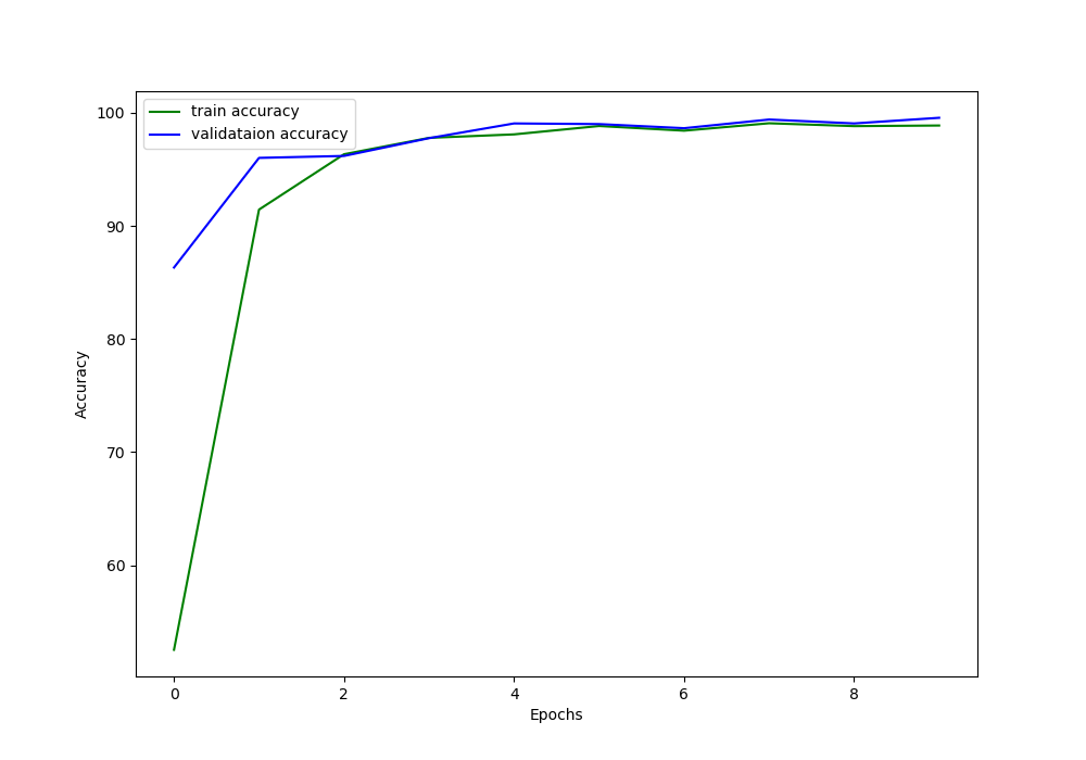
In figure 4, you can see that after the second epoch, the training accuracy and loss values are following closely. This is a good thing for our neural network model. Both, the training and validation accuracy values remain above 90% till the end of training. By the end we are getting more than 98% accuracy which great by the comparison of how simple our deep learning model is. Let’s just hope that this is not the case of overfitting on the data.

Now, let’s take a look at the loss value graph.

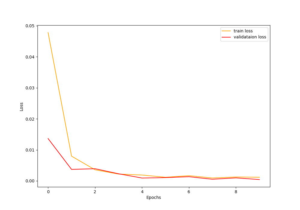
Figure 5 shows the loss values of training and validation for 10 epochs. The loss values also appear really good. Both, the validation loss and training loss are following closely. We are reaching near-zero loss by the end of the training.

Testing the Neural Network Model for American Sign Language Recognition

In this section, we will write the code to test our neural network model on the test images. Before moving further, you can take a look at the test images. They are inside input/asl_alphabet_test/asl_alphabet_test/.

All of the code in this section will go into the test.py python file.

Let’s start with importing the modules and building the argument parser.

'''
USAGE:
python test.py --img A_test.jpg
'''

import torch
import joblib
import torch.nn as nn
import numpy as np
import cv2
import argparse
import albumentations
import torch.nn.functional as F
import time
import cnn_models

# construct the argument parser and parse the arguments
parser = argparse.ArgumentParser()
parser.add_argument('-i', '--img', default='A_test.jpg', type=str,
    help='path for the image to test on')
args = vars(parser.parse_args())

We will give the image file name that we want the neural network model to test on as the command line argument.

Next, we will define image augmentation. Again, we will just apply resizing to the image.

aug = albumentations.Compose([
                albumentations.Resize(224, 224, always_apply=True),
])

Loading the Binarized Labels and the Trained Model

Now, we will load the binarized labels. After testing the model on a test image, we will get a single value. We will provide this value as the index to the label binarizer. And the value at that index will be our class label. This is a very easy and efficient way to track the predicted labels in deep learning and neural network training while testing the model.

# load label binarizer
lb = joblib.load('../outputs/lb.pkl')

Next, we will load our neural network model.

model = cnn_models.CustomCNN().cuda()
model.load_state_dict(torch.load('../outputs/model.pth'))
print(model)
print('Model loaded')

PyTorch provides the load_state_dict() function which is very useful in deep learning. First, at line 1, we initialize CustomCNN() model as usual. Then we use the load_state_dict() function at line 2 to load the trained weights from the model.pth file. This becomes very helpful when we are using transfer learning in deep learning and want to load the weights just for the trained layers.

Load and Prepare the Image for Testing

Here, we will load the image that we get from the command line argument. Then we will apply the agumentation, transform the image into a torch tensor and move the image to the GPU for testing.

Note that if you have trained the neural network model on the CPU, then move the image tensor to the CPU instead of the GPU.

image = cv2.imread(f"../input/asl_alphabet_test/asl_alphabet_test/{args['img']}")
image_copy = image.copy()
 
image = aug(image=np.array(image))['image']
image = np.transpose(image, (2, 0, 1)).astype(np.float32)
image = torch.tensor(image, dtype=torch.float).cuda()
image = image.unsqueeze(0)
print(image.shape)

Predict the Image Class and Visualize the Output Using OpenCV

Next, we need to predict the output (class) of the image. After predicting the class, we will also visualize the image on the screen with the class label showing on the image. We will use OpenCV for this. Along with that we will also save the predicted class label and image visualization to the outputs folder on the disk.

start = time.time()
outputs = model(image)
_, preds = torch.max(outputs.data, 1)
print('PREDS', preds)
print(f"Predicted output: {lb.classes_[preds]}")
end = time.time()
print(f"{(end-start):.3f} seconds")
 
cv2.putText(image_copy, lb.classes_[preds], (10, 30), cv2.FONT_HERSHEY_SIMPLEX, 0.9, (0, 0, 255), 2)
cv2.imshow('image', image_copy)
cv2.imwrite(f"../outputs/{args['img']}", image_copy)
cv2.waitKey(0)

Execute the test.py file using the following command. We will test on the A_test.jpg image.

python test.py --img A_test.jpg

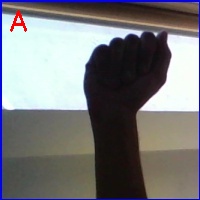
Looks like our neural network model has learned well. It is correctly classifying the sign language for the letter A.

Now, let’s try something a bit more complicated. The sign language for the alphabet S looks a lot like the alphabet A. So, let’s try our neural network model on the image of letter S.

python test.py --img S_test.jpg

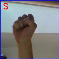
Our deep learning model is correctly classifying the alphabet S as well. It seems that the neural network has not overfit while training after all.

Next, we will write the code to perform sign language detection using webcam in real-time.

Performing Sign Language Recognition in Real-Time from Webcam Feed

OpenCV provides very easy setup for connecting our python code and reading and frames from the webcam. For this part, you will need a webcam connected to your computer.

All of the code in this section will go into cam_test.py file. Let’s start with importing the required modules, loading the binarized labels, and loading the trained neural network model as well.

'''
USAGE:
python cam_test.py 
'''

import torch
import joblib
import torch.nn as nn
import numpy as np
import cv2
import torch.nn.functional as F
import time
import cnn_models
 
# load label binarizer
lb = joblib.load('../outputs/lb.pkl')

model = cnn_models.CustomCNN().cuda()
model.load_state_dict(torch.load('../outputs/model.pth'))
print(model)
print('Model loaded')

Helper Function to Capture Hand Area

Here, we will define a simple function to capture a rectangular area on the webcam frame. There are a few reasons for doing this.

• We do not want our neural network model to detect images from the whole webcam frame.
• We only want the neural network to get activated when we show our hand signs in a particular area on the screen.
• The hand sign needs to appear in this rectangular area.
• The network will predict the alphabet if it sees a hand sign in this rectangular region only.

def hand_area(img):
    hand = img[100:324, 100:324]
    hand = cv2.resize(hand, (224,224))
    return hand

So, this rectangular region is a 224×224 dimensional region. It is the same size as the images on which our neural network model has been trained.

Capture the Webcam

We need to capture the webcam frames using OpenCV. For this, we can use the OpenCV VideoCapture(). We will create a VideoCapture() object.

cap = cv2.VideoCapture(0)

if (cap.isOpened() == False):
    print('Error while trying to open camera. Plese check again...')

# get the frame width and height
frame_width = int(cap.get(3))
frame_height = int(cap.get(4))

# define codec and create VideoWriter object
out = cv2.VideoWriter('../outputs/asl.mp4', cv2.VideoWriter_fourcc(*'mp4v'), 30, (frame_width,frame_height))

• At lines 7 and 8, we get the frame height and width.
• Then we create a VideoWriter() object and define the codec for saving the webcam frames (line 11).

Reading the Frames and Predicting the Output in Video Feed

We will keep capturing the webcam frames until the user presses q key on the keyboard.

The following code shows how to do this.

# read until end of video
while(cap.isOpened()):
    # capture each frame of the video
    ret, frame = cap.read()
    # get the hand area on the video capture screen
    cv2.rectangle(frame, (100, 100), (324, 324), (20, 34, 255), 2)
    hand = hand_area(frame)

    image = hand
    
    image = np.transpose(image, (2, 0, 1)).astype(np.float32)
    image = torch.tensor(image, dtype=torch.float).cuda()
    image = image.unsqueeze(0)
    
    outputs = model(image)
    _, preds = torch.max(outputs.data, 1)
    
    cv2.putText(frame, lb.classes_[preds], (10, 30), cv2.FONT_HERSHEY_SIMPLEX, 0.9, (0, 0, 255), 2)
    cv2.imshow('image', frame)
    out.write(frame)

    # press `q` to exit
    if cv2.waitKey(27) & 0xFF == ord('q'):
        break

# release VideoCapture()
cap.release()

# close all frames and video windows
cv2.destroyAllWindows()

• At line 6, we draw a red rectangular area on the screen as a prompt for the user for where to show the hand.
• Then we get the area image at line 7 and treat it as an image (line 9).
• After that all the steps are similar to recognizing the hand signs on images. Instead of images, we do that on each webcam frames.
• You can press q on the keyboard to exit the webcam feed.

Executing the cam_test.py file

Let’s execute the cam_test.py file and try out some real-time American Sign Language Recognition.

python cam_test.py

After executing the python file, you should see the webcam getting activated. You can place your hand with a sign language letter within the red rectangular region and the neural network model will try to predict the alphabet.

Below I am showing a short clip of the output of the real-time American Sign Language recognition that has been saved to the disk.

The model is doing good at predicting the letters. But still, we can see a lot of fluctuation in the real-time predictions. Even a slight hand movement is making the neural network change its predictions. This is also called as ‘flickering‘.

You can carry on from here on and try to make the model better and more robust to such fluctuations. I would recommend you search the internet and find out some ways to correct this. If you find a good method and improve on this, then do share your findings in the comment section. I will surely address that.

Summary and Conclusion

In this article, you learned how to train a neural network for American Sign Language recognition. We used deep learning. In specific you learned:

• How to use a subset of a large image dataset for training a deep neural network.
• Recognizing American Sign Language from images.
• Real-time recognition of American Sign Language from webcam feed.

I hope that you learned a lot from this tutorial. Do leave your thoughts and doubts in the comment section, and I will try my best to address them.

You can contact me using the Contact section. You can also find me on LinkedIn, and Twitter.