Edge Detection in Computer Vision using OpenCV

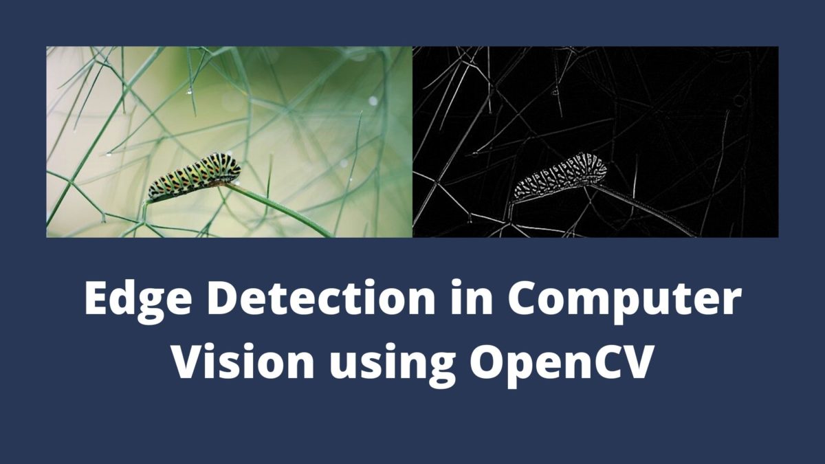
In this tutorial, you will learn how to perform edge detection in computer vision using the OpenCV library. In the field of computer vision and machine learning, edge detection is a very fundamental problem and has a wide variety of applications.

What will we cover in this tutorial?

• Introduction to edge detection in computer vision.
  • What is edge detection and why do we need it?
• Different types of edge detection algorithms:
  • Sobel edge detection.
  • Laplacian edge detection.
  • Canny edge detection.
• Using OpenCV to highlight edges in images.
• Highlighting edges in videos using OpenCV.

Introduction to Edges and Edge Detection in Computer Vision

As humans, we can easily recognize objects by seeing a colored pictures. But not only that, we can very easily detect and recognize objects just from the outline of an object or image. When the edges are defined, then we can easily conclude the type of object we are seeing.

So, the real question is, can computer systems also detect edges of the objects easily? The short answer is yes.

In an image, when we encounter an edge, then there is a very sharp change in the pixel intensities of the image. In the field of computer vision, mathematically, an edge leads to change in derivatives of the pixels.

So, to detect edges in images, we need to track down these sharp changes in pixel intensities.

Why Edge Detection in Computer Vision?

Now, what is the motivation behind carrying out edge detection of images?

Detecting edges in images may lead to capturing some important changes that have taken place. Some of those include:

• If there is a change in lighting and illumination?
• Changes in the depth of the image scene.
• Whether there are any changes in material properties?

There is another very important reason behind edge detection. Detecting just the edges reduces a lot of background noise, thus revealing the required and important changes in the real world.

How do We Carry Out Edge Detection in Computer Vision?

To carry edge detection, we use a kernel or filter that we pass over the image. This kernel contains some real-valued integers which help in carrying out the process of edge detection.

The process of applying the kernel operation over the image is called convolution. In computer vision, convolution is a very fundamental operation which can help in blurring, deblurring, and detecting edges images as well.

We will not go very deep into the concepts of kernel and convolution in this tutorial. You can read this tutorial to know more about kernels and convolutions. You will also get to learn how to blur images using different kernels.

Now, let’s move to different types of edge detection techniques in computer vision.

The Sobel Edge Detector

The Sobel edge detection algorithm is quite well known within the computer vision community. It is a very widely used edge detection technique. We need not go much into the historical details, but still, it is named after Irwin Sobel and Gary Feldman who created this algorithm at the Stanford Artificial Intelligence Laboratory (SAIL).

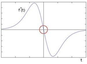
The Sobel edge detector works by computing the gradient of the pixel intensities of an image.

So, if there is an edge present in the image, then there will be a jump in the intensity of the plot.

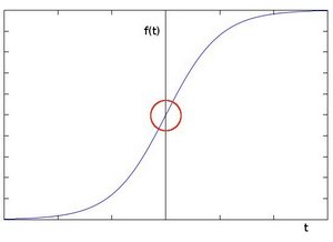
In figure 1, the circle indicates a change in the pixel intensity in the image.

Now, if we take the derivative of the above plot, then the intensity change will show as the point of maximum in the plot.

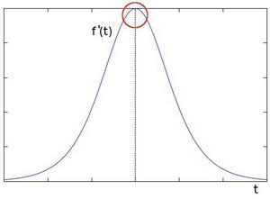
So, if the gradient is higher than a threshold, we can conclude that there is an edge present in the image.

In the Sobel operation, we need to carry out the convolution operation. We need to convolve an image using a filter or kernel. This filter contains integer values. During the convolution of the image with the Sobel filter, it can be either in the vertical or the horizontal direction.

The Working of Sobel Edge Detector

In this section, we will learn how the Sobel edge detector actually works.

The Sobel edge detector uses two 3×3 kernels. These two kernels are convolved with an image to calculate the approximations of the derivative.

One of the kernels is used for computing the vertical gradient approximations. The other kernel is used for computing the horizontal gradient approximations. Typically, we can say that, one for the x-direction, and the other for the y-direction.

But, how do we calculate the horizontal and vertical changes? The following explanation should clear this up.

Let \(I\) be the source image on which we want to carry out the Sobel operation.

For the Vertical Derivatives

We need to convolve the image ​ with a kernel. Now, this kernel needs to be an odd-shaped matrix. Let’s take a 3×3 example.

Let the kernel for the vertical derivatives be

$$
\begin{bmatrix} +1 & 0 & -1\\ +2 & 0 & -2\\ +1 & 0 & -1\end{bmatrix}
$$

Supposing that \(G_x\) ​gives the vertical gradient approximations.

$$
G_x = \begin{bmatrix} +1 & 0 & -1\\ +2 & 0 & -2\\ +1 & 0 & -1\end{bmatrix} * I
$$

In the above formula, ​ \(*\) denotes the convolution operation.

For the Horizontal Derivatives

Let the kernel for horizontal derivatives be

$$
\begin{bmatrix}
+1 & +2 & +1\\
0 & 0 & 0\\
-1 & -2 & -1\end{bmatrix}
$$

Now, \(G_y\)​ gives the horizontal gradient approximations.

$$
G_y = \begin{bmatrix}
+1 & +2 & +1\\
0 & 0 & 0\\
-1 & -2 & -1\end{bmatrix} * I
$$

The x-coordinate and the y-coordinate both move and increase in the right and downward directions respectively. Next, we can combine the gradient magnitude to get the resulting gradient at each point in the image.

$$
G = \sqrt{G_x^2 + G_y^2}
$$

Let’s take look at some Sobel edge highlighting examples: (The images are from Wikipedia).

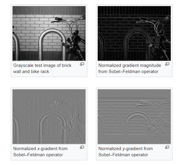
In figure 3, you can see how the x and y gradients capture different edges respectively. And the final Sobel detection is an addition of the weighted average of the two x and y direction gradients.

Now, we will learn about two more edge detector algorithms. We will not go much into the theoretical details of these two. Instead after a short explanation of the two, we will move onto the coding part, which will give a much better perspective of the working of the detectors.

The Laplacian Edge Detector

In the Sobel edge detector, the first order derivative of the pixel intensities shows a jump in the pixel intensities. This in turn indicates the presence of an edge in the image.

Now, when we take the second-order derivative, then we get 0 (zero). And this is the concept behind the Laplacian edge detector algorithm in computer vision.

The Laplacian edge detector uses only one kernel. The formula for the edge detector is:

$$
Laplace(f) = \frac{\partial^{2} f}{\partial x^{2}} + \frac{\partial^{2} f}{\partial y^{2}}
$$

We will not go into more details of the Laplacian theory, but you can find a really detailed one here.

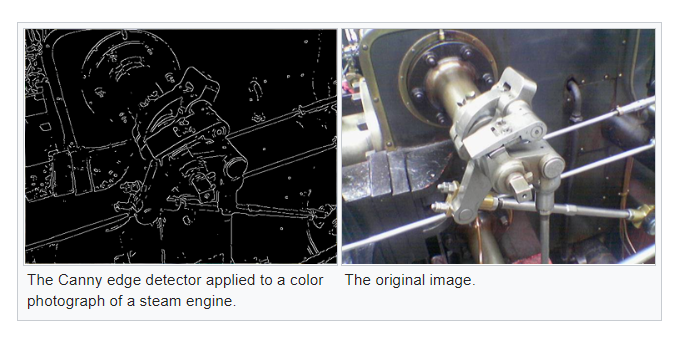
The Canny Edge Detector

The Canny edge detection algorithm was developed by John F. Canny in 1986.

The following is an example image from Wikipedia.

The Working of Canny Edge Detector

The following are very high level steps of computing the edge in an image using the Canny edge detector.

• Apply the Gaussian filter to smooth the image in order to remove the noise.
• Find the intensities of the gradients of the image in the x-direction and y-direction. This step is similar to finding \(G_x​\) and \(G_y\) ​in the Sobel edge detection.
  • Then find the resulting gradient: ​\(G = \sqrt{G_x^2 + G_y^2}\).
• Apply non-maximum suppression to get rid of the parts that are not the edges of the image.
• Then we track edge hysteresis:
  • Accept a pixel as an edge if the pixel gradient is higher than a pixel threshold.
  • Reject a pixel if the pixel gradient is lower than the pixel threshold.
  • If the pixel gradient is in between, then accept only if the pixel is connected to a higher than upper threshold pixel.

If you want to get into the details, then you can find more information here.

Now, let’s move onto the coding part of the tutorial.

Edge Detection in Computer Vision using OpenCV

Beginning from this section, we will focus on the coding part. You will learn:

• Applying different edge detectors to images:
  • Sobel edge detector to images.
  • Laplacian edge detector to images.
  • Canny edge detector to images.
• Applying the Laplacian edge detector on videos.

Before that, let’s take a look at the directory structure. You will find the tutorial a lot easier to follow, if you use the same structure as well.

│   highlight_edges.py
│   highlight_edges_vid.py
│
├───edges
│       caterpillar_canny.jpg
|         ...
│
├───images
│       caterpillar.jpg
│       meerkat.jpg
│
└───videos
        rose.mp4

• We have two python files, highlight_edges.py for detecting edges in images, and highlight_edges_vid.py for detecting edges in videos.
• The edges folder will contain all the outputs images and videos that we will save while running the python files.
• The images folder contains two images, caterpillar.jpg, and meerkat.jpg that we will use to apply the edge detection algorithms.
• videos folder contains rose.mp4 video. We will use this video to apply the edge detectors.

You can use any images and videos of your choice for this tutorial. Still, if you want the use the same as shown here, then the following are the links:

• Caterpillar image.
• Meerkat image.
• Rose video.

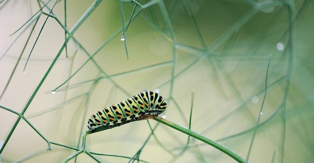
In this tutorial, we will apply the edge detection algorithms to the caterpillar image only. This will help us better compare the results of the different edge detectors that we will write the code for. You can try out the meerkat image yourself and let me know the findings in the comment section.

Applying Edge Detectors to Images

From here, on we will write the code to apply different edge detectors to the images. All of the code from hereon will go into the highlight_edges.py file.

Importing Modules and Building Argument Parser

In this section, we will import all the required modules and build the argument parser to parser the command line arguments.

import cv2
import argparse

# build argument parser and parser command line arguments
parser = argparse.ArgumentParser()
parser.add_argument('-i', '--image', type=str, default='caterpillar.jpg', 
                    choices=['caterpillar.jpg', 'meerkat.jpg'])
parser.add_argument('-e', '--edge', default='sobel', 
                    choices=['sobel', 'laplacian', 'canny'])
parser.add_argument('-b', '--blur' , default='yes', 
                    choices=['yes', 'no'])
args = vars(parser.parse_args())


img = cv2.imread(f"images/{args['image']}")

We only need the OpenCV and argparse modules.

For the argument parsers:

• --image gives the image file name to use for edge detection.
• --edge will give the edge detection algorithm to use on the image. There are three choices, ['sobel', 'laplacian', 'canny'].
• --blur decides whether we apply Gaussian blurring to the image or not. By default, it is yes.

Applying blurring to the image is important while carrying edge detection in computer vision. This is because blurring helps to remove most of the background noises. This helps the edge detection algorithm to focus on detecting the edges.

Finally, at line 15, we read the image file that we provide as the command line argument.

Applying Sobel Edge Detector to Images

Here, we will add the code to apply the Sobel edge detector to the images.

The following code block shows how to add Sobel edge detector to an image using OpenCV and python.

# sobel
if args['edge'] == 'sobel':
    if args['blur'] == 'yes':
        img = cv2.GaussianBlur(img, (3, 3), 0) # to reduce the noise
    img_gray = cv2.cvtColor(img, cv2.COLOR_BGR2GRAY)
    gx = cv2.Sobel(img_gray, cv2.CV_32F, 1, 0, ksize=3) # the x - direction gradient
    gy = cv2.Sobel(img_gray, cv2.CV_32F, 0, 1, ksize=3) # the y - direction gradient
    sobel_final = cv2.addWeighted(gx, 0.5, gy, 0,5, 0) 
    cv2.imwrite(f"edges/{args['image'].split('.')[0]}_sobel_gx.jpg", gx)
    cv2.imwrite(f"edges/{args['image'].split('.')[0]}_sobel_gy.jpg", gy)
    cv2.imwrite(f"edges/{args['image'].split('.')[0]}_sobelfinal.jpg", sobel_final)
    cv2.imshow('Sobel G_x', gx)
    cv2.imshow('Sobel G_y', gy)
    cv2.imshow('Sobel Weighted', sobel_final)
    cv2.waitKey(0)

The above code will execute if we give --edge sobel while executing the python file. And the Gaussian blurring will be applied to the image by default.

• First, at line 4, we apply Gaussian blurring to the image with kernel size 3×3.
• Line 5, converts the image to grayscale. Converting the image to grayscale is not necessary, but we are doing it here. You can also check without converting the image to grayscale.
• Lines 6 and 7, find the x-direction and y-direction gradients respectively. We use the OpenCV Sobel function for that.
  • It first takes the image as an argument.
  • Then we imply to convert the pixels to 32-bit float.
  • 1, 0 indicates that we want to calculate the x-direction gradients. And 0, 1 for the y-direction gradients.
  • The final argument is the kernel size, that we have given as 3.
• At line 8, we use OpenCV addWeigted() to get the weighted sum of gx and gy. The two 0.5 values indicate the weights of gx and gy respectively. The final 0 is the gamma argument which is a scalar weight added to each sum.
• Then from lines 9 to 14, first we are saving all the three images according to the image file that we are using. We are saving the images in the edges folder. Finally, we are showing the images on the screen.

Now, you can execute the python file by typing the following command in the terminal.

python highlight_edges.py --edge sobel

You will find the following images saved in the edges folder.

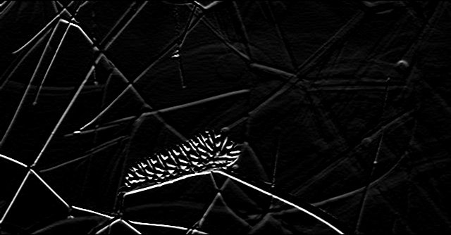
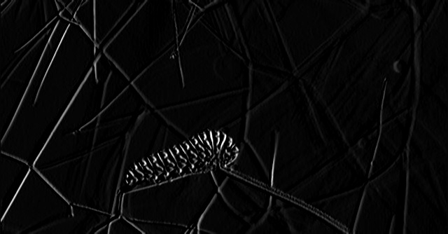
In figure 8, you can see that the image shows most of the vertical lines. This is because this image shows the x-direction gradients which captures the vertical direction gradients. In the same way, figure 9 captures all the horizontal gradients. And figure 10 shows the weighted average of both the gradients.

You can also try and execute the python file with the meerkat.jpg file to get a better perspective of the gradient directions.

Applying the Laplacian Edge Detector

Here, we will apply the Laplacian edge detector to the image.

The following is the code that applies Laplacian edge detector to an image.

# laplacian
if args['edge'] == 'laplacian':
    if args['blur'] == 'yes':
        img = cv2.GaussianBlur(img, (3, 3), 0) # to reduce the noise
    img_gray = cv2.cvtColor(img, cv2.COLOR_BGR2GRAY)
    laplacian = cv2.Laplacian(src=img_gray, ddepth=cv2.CV_8U, ksize=3)
    cv2.imwrite(f"edges/{args['image'].split('.')[0]}_laplacian.jpg", laplacian)
    cv2.imshow('Laplacian edge', laplacian)
    cv2.waitKey(0)

As usual, we blur the image first and convert the image to grayscale.

• At line 6, we apply the Laplacian edge detector to the image. We have provided three arguments to the function.
  • First is src, the source image.
  • Second one is ddepth which is the desired depth of the destination image. We have given the ddepth as CV_8U which corresponds to 8-bit unsigned values.
  • The final argument is the ksize. This is Laplacian kernel size which is 3 in our case.
• Then we save the image to disk and show the image on the screen.

Let’s execute the python file to apply Laplacian edge detector to the caterpillar image.

python highlight_edges.py --edge laplacian

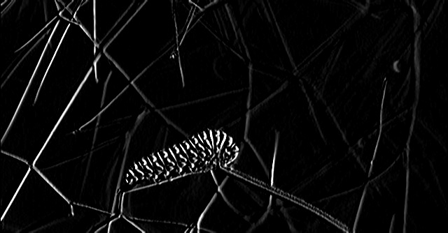
The following is the image that you will find in the edges folder.

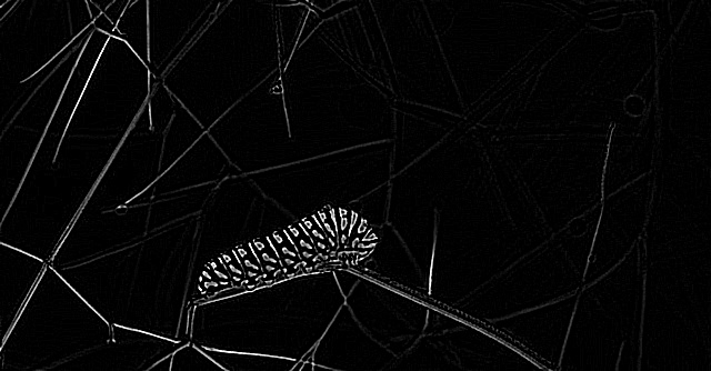
In figure 11, you can see that the edges of the image are very well defined. The patterns on the body of the caterpillar and the twigs behind are all very sharp. In fact, if you compare the image with Sobel edge detection results, then you will find that the edges of the Laplacian detector are much sharper.

Applying the Canny Edge Detector to the Image

In this section, we will apply the Canny edge detector to the caterpillar image.

Again, OpenCV makes the work much easier for us. The following is the code for applying the Canny edge detector to an image.

# canny
if args['edge'] == 'canny':
    if args['blur'] == 'yes':
        img = cv2.GaussianBlur(img, (3, 3), 0) # to reduce the noise
    img_gray = cv2.cvtColor(img, cv2.COLOR_BGR2GRAY)
    canny = cv2.Canny(img_gray, 100, 200)
    cv2.imwrite(f"edges/{args['image'].split('.')[0]}_canny.jpg", canny)
    cv2.imshow('Canny', canny)
    cv2.waitKey(0)

• First we apply Gaussain blurring to the image and convert the image to grayscale at lines 4 and 5.
• Then at line 6, we use the OpenCV Canny() function.
  • The first argument is the source image as usual.
  • The second and third arguments are the lower and higher thresholds to accept a pixel for detecting edges.
  • In our case, if the pixel gradient is higher than 200, then we will consider it for detecting edges. If the pixel gradient is less then 100, then we will reject it. If the value is between 100 and 200, then we accept if the pixel is connected to another pixel whose gradient is higher than 200.
• Finally, we save the image to disk and show the image on the screen.

Execute the Canny edge detector.

python highlight_edges.py --edge canny

You will find the following image in the edges folder.

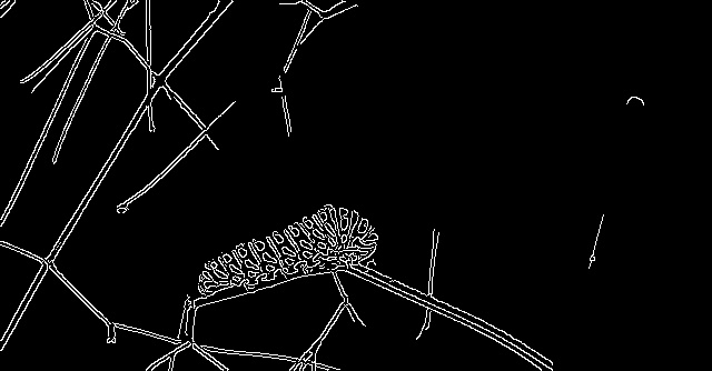
You can see that the edges are really sharp, even sharper than the Laplacian edge detector. But the detector is missing some edges of the twigs which were present in both, Laplacian and Sobel edge detectors.

Now, you will find that executing the Canny edge detector without the Gaussian blurring, includes a lot of pixel noise on the twigs. Do give it a try on your own. Gaussian blurring helps a lot in this case.

Next, we will move onto applying edge detection algorithms to videos using OpenCV.

Applying Edge Detection to Videos

In this section, we will write to the code to apply the Laplacian edge detector to the rose.mp4 file that we have inside the videos folder. Feel free to use any other video of your choice.

Using OpenCV, it is very easy to work with videos. All of the code from this section will go into the highlight_edges_vid.py file.

Imports and Reading the Video File

Let’s import the modules that we require and read the video file that we will work upon.

import cv2

cap = cv2.VideoCapture('videos/rose.mp4')

if (cap.isOpened() == False):
    print('Error while trying to read frames. Please check again...')

# get the frame width and height
frame_width = int(cap.get(3))
frame_height = int(cap.get(4))
vid_codec = cv2.VideoWriter_fourcc(*'mp4v')

# define codec and create VideoWriter object
out = cv2.VideoWriter(f"edges/laplacian_vid_edge.mp4", vid_codec, 30, (frame_width, frame_height))

In the above code block:

• We read the video file at line 4 and check for error at line 6.
• Lines 9 and 10get the height and width of the video frame.
• Line 11 defines the video format to save the video file.
• At line 15, we define a VideoWriter() object and define the codec for saving the frames later on.

Reading Video Frames and Applying the Laplacian Edge Detector

We will read the video file until the end and apply the Laplacian edge detector to each of the frames. We will not apply the Gaussian blurring here. You can however add Gaussian blurring if you wish to.

The following code block shows how to read the frames and apply the Laplacian edge detection.

# read until end of video
while(cap.isOpened()):
    # capture each frame of the video
    ret, frame = cap.read()
    if ret == True:
        frame = cv2.Laplacian(src=frame, ddepth=cv2.CV_8U, ksize=3)
        # save video frame
        out.write(frame)
        # display frame
        cv2.imshow('Video', frame)

        # press `q` to exit
        if cv2.waitKey(27) & 0xFF == ord('q'):
            break
    else:
        break

# release VideoCapture()
cap.release()

# close all frames and video windows
cv2.destroyAllWindows()

• At line 6, we are applying the Laplacian edge detector to each of the read frames. The kernel size is 3.
• We then save the frame at line 8 and display the frame at line 10.
• After reading all of the frames, we release the VideoCapture() object and destroy all video windows.

Execute the file by typing the following command in the terminal.

python highlight_edges_vid.py

You will find laplacian_vid_edge.mp4 file inside the edges folder.

The output is pretty amazing. You can have a lot of fun with new videos.

One thing that you can try out is combining such edge detection techniques and other computer vision based deep learning ideas. I think that combining ideas and building something will lead to an amazing project in the end.

Summary and Conclusion

In this tutorial, you learnt:

• The theory of edge detection in the field of computer vision.
• Detecting edges using OpenCV and different algorithms like Sobel, Laplacian, and Canny edge detectors.
• Detecting edges in videos using OpenCV.

If you have any thoughts or doubts, then you can leave them in the comment section and I will try my best to address them.

You can contact me using the Contact section. You can also find me on LinkedIn, and Twitter.