Image Recognition using Histogram of Oriented Gradients (HOG) Descriptor

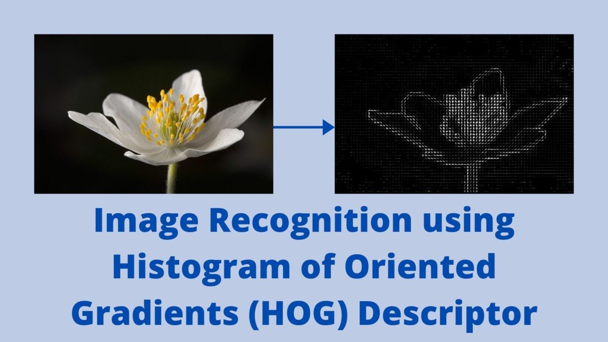
In this post, you will learn about the Histogram of Oriented Gradients (HOG) descriptor in the field of computer vision. Along with that, you will also learn how to carry out image recognition using Histogram of Oriented Gradients (HOG) descriptor and Linear SVM.

A bit of background…

I constantly learn about deep learning and do projects about the things that I learn as well. At the same time I write about the things that I am learning here at DebuggerCafe. In deep learning and computer vision, object detection is one of the most active topics. While trying to learn about object detection, I stumbled upon the HOG feature descriptor. This is one of many traditional computer vision and machine learning techniques that we can use for object detection. And quite frankly, it is a great topic in computer vision to learn about as well.

Although we will not be learning about object detection using the HOG descriptor in this post, we will learn about image recognition using Histogram of Oriented Gradients. And before doing that, let’s learn about some of the important concepts of the HOG descriptor.

The HOG Feature Descriptor

We get really great results when we combine computer vision and machine learning techniques. Let’s start with the definition of the HOG feature descriptor.

HOG is a feature descriptor for images that we can use in computer vision and machine learning. It is widely used in vision and image processing tasks for object detection and recognition.

It was developed by Dalal and Triggs in 2005. As of 2020, the paper may be 15 years old, but it is still used in the industry for object detection and computer vision tasks. The main reason is that it is accurate and fast. Although it may not be as good as today’s deep learning object detection techniques, still it is fairly fast and we can easily run the program on a CPU.

HOG feature descriptor by Dalal and Triggs combines two techniques. Those are computer vision and machine learning. They combine fine-scale gradient computation techniques from the field of computer vision and used the Linear SVM machine learning technique to create an object detector. In short, the gradient intensities of an image can reveal some useful local information that can lead to recognition of the image.

The main highlight of the paper is the HOG feature descriptor. But what is a feature descriptor actually?

Feature Descriptor

Basically, we can define an image by the pixel intensities and intensities of the gradients of the pixels. These gradients work in the same way as they in detecting edges in images. You can have a better understanding of edge detection from this post.

So, a feature descriptor tries to capture the important information in an image and keeps all the not-so-important information behind the scenes. Then we can use the useful information from the feature descriptor for image recognition and object detection.

As we discussed in the edge detection post, detecting edges can many times lead to recognizing the objects easily. This is because the outline of an image gives a lot of information about what the image can be. In the HOG descriptor, this corresponds to the gradient computation step that we will take look at shortly.

A Little Bit of Code to Show a Feature Descriptor using HOG

All the theories will not do any good if we do not know how to implement them and what results it will produce. After all, what does a feature descriptor look like?

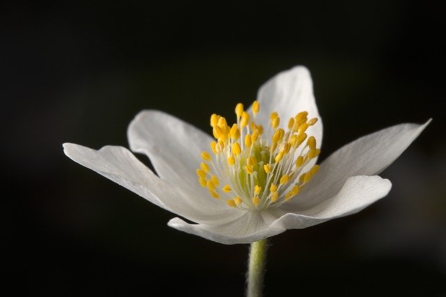
In this section, we will see a very small code snippet to visualize the feature descriptor using HOG. You will need Scikit-Image to run this code and further along in this article as well. So, install it if you do not have it already. You can try any image you want. I will be using the following flower image. You can save it if you want.

The Python Code

from skimage import feature
import cv2
import matplotlib.pyplot as plt

image = cv2.imread('flower.jpg')
(hog, hog_image) = feature.hog(image, orientations=9, 
                    pixels_per_cell=(8, 8), cells_per_block=(2, 2), 
                    block_norm='L2-Hys', visualize=True, transform_sqrt=True)

cv2.imshow('HOG Image', hog_image)
cv2.imwrite('hog_flower.jpg', hog_image*255.)
cv2.waitKey(0)

First, we import the feature module from skimage. Then we read the image. At line 6, we use feature.hog() function to calculate the HOG features. You can see that it returns two values that we are capturing. One is hog and the other is hog_image. The original descriptor is hog. And hog_image is the descriptor image that we can visualize. It returns the second value (hog_image in our case) only of the visualize argument is True in feature.hog(). Else it only returns the first value only (that is hog).

Running the above python script with give the following output.

python hog_flower.py

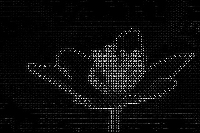
You can see that the image intensities around the flower are much more pronounced than the background. Local information like these actually help the HOG feature descriptor to carry on image recognition.

Now, in the above code, we use the feature.hog() function. But we did not go through all the arguments in detail. The output you see above is the final descriptor. There are many intermediary steps. You will get a better understanding of all the arguments once we learn about the steps of calculating the HOG feature descriptor.

The 5 Steps of HOG Feature Descriptor

The 5 steps of the HOG Feature Descriptor are:

• Preprocessing (Gamma/Color Normalization and Resizing).
• Computing the Gradients.
• Spatial / Orientation Binning (Dividing the image into cells).
• Block Normalization.
• Get the HOG Feature Vector.

All of these steps are as implemented in the original paper. I will try to keep them as brief and easy to understand as possible.

Step 1: Gamma / Color Normalzation

Image preprocessing and color normalization are typical of any computer vision tasks. It may be any traditional methods or deep learning methods, image resizing and normalizing the pixels values are very important steps.

For the HOG feature descriptor, the most common image size is 64×128 (width x height) pixels. The original paper by Dalal and Triggs mainly focused on human recognition and detection. And they found that 64×128 is the ideal image size, although we can use any image size that has the ratio 1:2. Like 128×256 or 256×512.

Next is choosing between color scales and color normalization. The authors say that both RGB and LAB color spaces perform identically. But using grayscale images reduces performance. This means that HOG feature descriptor works best on colored images.

Step 2: Computing the Gradients

The next step is calculating the image gradients. To learn more about image gradients, you can take a look at my edge detection post.

Typically, computing the gradients of an image in computer vision reveals those locations where the pixel gradient intensities change. Thus, this leads to a lot of useful information.

In the research, the kernels used to calculate the gradients are:

• Vertical gradient kernel: \([-1, 0, 1]\)
• Horizontal gradient kernel: \(\begin{bmatrix} -1\\ 0 \\ 1\end{bmatrix}\)

Let \(G_x\) and \(G_y\) be the vertical and horizontal gradients respectively. Then the final gradient magnitude is:

$$
G = \sqrt{G_x^2 + G_y^2}
$$

Let’s take a look at the flower image after applying the kernels and calculating the gradients.

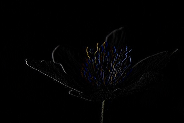
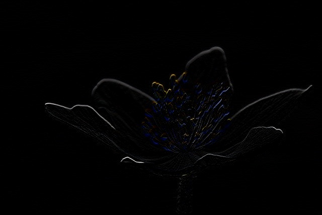
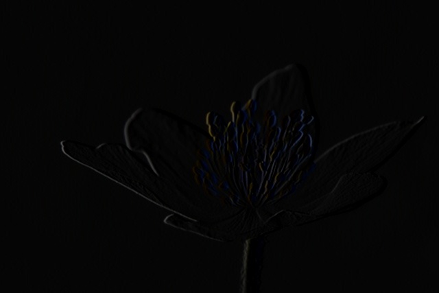
Figure 4 shows the horizontal direction gradients, figure 5, shows the vertical direction gradients, and figure 6 shows the final magnitude of the two. You can achieve the above results by applying the Sobel operator in OpenCV with a kernel size of 1. Again, you can find about the Sobel operator in this post in much more detail.

Step 3: Spatial / Orientation Binning and Calculating the Gradients

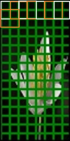
The next step is dividing the image into 8×8 cells. Then we calculate the gradients for all the 8×8 cells.

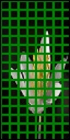
Figure 7 shows the result of dividing the flower image into 8×8 cells. So, if it is a 64×128 dimensional image, then there would be 8 cells in the horizontal direction for each row. And there would be 16 cells in the vertical direction for each column. Each cell has 8x8x3 = 192 pixels. And the gradient of each cell has the magnitude and direction (2 values). So, each cell has 8x8x2 = 128 values as the gradient information.

The gradients and directions are each 8×8 blocks containing numbers. They are represented using 9 orientation bins.

The following image shows an example of 9 bin values in the form of a histogram.

Figure 8 shows the bin values for one of the grid cells in figure 7. So, we get 128 such bin value histograms in total for a total of 128 cells in the image. You can see that most of the bins are empty. This is mostly because, these bins represent the first grid cell, where the image does not contain much gradient information.

Now, let’s move on to the next step.

Step 4: Block Normalization

In the previous step, we divide the image into grids of 8×8 cells and calculate the gradients for each cell. According to the authors of the paper, gradient values can vary according to the lighting and foreground & background contrast.

So, to counter this issue, we can normalize the cells. In such cases, block normalization tends to perform better than single-cell normalization. We will group a few cells together and normalize the gradient values of each block (grouped cell).

In figure 9, you can see that we have grouped 4 cells together to make a block. We call this as 2×2 block normalization. You can also use 3×3 block normalization where you group 9 cells together. The authors find that both, 2×2 block normalizations and 3×3 block normalization work well.

There is another catch here. In all cases, there is an overlap of 2 cells. So, the stride of the blocks is one. According to the authors, fixing the stride to half the block size will yield good results. This results in each cell contributing to the normalization process more than once. The authors find that L1-sqrt, L2-norm, and L2-Hys, all three normalizations perform identically and give good results. You may take a look at the paper to get a better idea about the normalization schemes.

Step 5: Getting the HOG Feature Vector

The final step is obtaining the HOG feature vector.

After we calculate all the block normalizations, we concatenate them into a single vector to get the final feature vector. There are 7 horizontal vectors and 15 vertical vectors. They amount upto a total of 105 vectors which are concatenated together to get the final feature vector.

After we get the final feature vector, we can use a machine learning algorithm like Linear SVM to carry on with image recognition.

Before Moving to the Image Recognition Coding Part…

In the above section, we discuss how the HOG feature descriptor works. But we did not go into the numbers and results that the authors mention in the paper. I think that reading that paper will give you a much better perspective of the numbers and results that the authors mention.

Still, before we move forward, let’s point out what works best while using the HOG feature descriptor. This is because we will try to use those recommended values in our coding.

According to the authors, the following values work best:

• 1D centered kernels or filters [-1, 0, +1].
• Image size is 64×128 (width x height).
• The cell size of 8×8. Each cell in the grid is 8 pixels x 8 pixels.
• Block size is 16×16 pixels (2×2 cells) => Take two 8×8 cells, both horizontally and vertically.

Just one more thing. Using the HOG feature descriptor for image recognition works best for those images which have a very defined and easily recognizable shape. Such images have gradients that give the most useful information. For example, the authors applied this to recognizing and detecting human images that have very defined gradient values. So, those images which cannot give good gradient values, HOG descriptor performs worse for those recognition tasks.

We will analyze such problems while coding our way through the image recognition part.

Image Recognition using Histogram of Oriented Gradients (HOG) Descriptor and Linear SVM

From this section, we will start our python coding. We will use HOG feature descriptor and Linear SVM to carry out image recognition.

For image recognition, we will use two sets of data. First, we will use a small flower dataset to train and predict on HOG features using Linear SVM. Then we will use another dataset consisting of humans, cars, and cups.

The Project Structure and the Dataset

Before moving further, let’s take a look at the project structure.

│   hog_image_recognition.py
├───input
│   ├───flowers
│   │   ├───daffodil
│   │   ├───lily
│   │   ├───rose
│   │   └───sunflower
│   └───person_car_cup
│       ├───car
│       ├───cup
│       └───person
├───outputs
└───test_images
    ├───flowers
    └───person_car_cup

• We have the hog_image_recognition.py which will contain our python code.
• Then, we have the input folder that will contain our two datasets, flowers and person_car_cup.
  • flowers has four subfolders and they contain the images of flowers according to their names. Those are daffodil flowers, lily flowers, rose flowers, and sunflowers. Each of the flower types contains 6 images
  • person_car_cup has three subfolders, car, cup, and person. Each folder has 5 images of the respective type.
• The outputs folder will save the outputs from running the python script.
• Finally, the test_images folder again has two subfolders with the names corresponding to the datasets.
  • The flowers subfolder contains one flower from each type. And the person_car_cup has one image from each type.

This is a very small dataset with only one python script. You can download the whole dataset and project here.

Now, let’s take a look at some of the images in the dataset. First, the following are the some of the flower images.

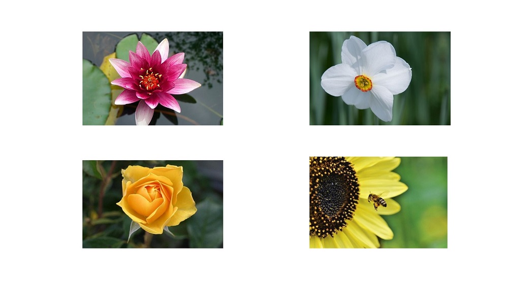
Figure 10 shows one flower from each type.

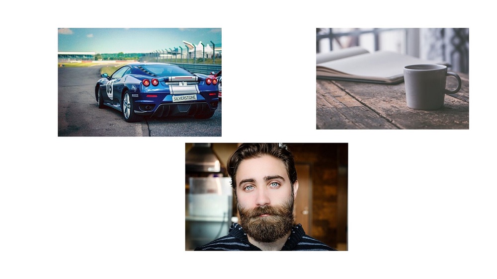
Figure 11 shows one image each from the input folder’s person, car, and cup category.

You can explore around and make yourself familiar with the data a bit more.

Writing the Python Script for Image Recognition using HOG Descriptor

We will write a single python script for training and predicting using a Linear SVM model on the two datasets. That means, we have to employ some methods with which we can just input the dataset name and our script will automatically train and predict on that.

Let’s start writing the code into hog_image_recognition.py file and see how we can arrange everything.

Importing the Modules

We will use the Scikit-Image implementation of the HOG feature descriptor in this tutorial. There is also an OpenCV implementation. But it is based more on the original paper and facilitates human recognition and detection. So, we will use Scikit-Image implementation.

'''
USAGE:
python hog_image_recognition.py --path person_car_cup
python hog_image_recognition.py --path flowers
'''

import os
import cv2
import argparse

from sklearn.svm import LinearSVC
from skimage import feature

We are importing feature module from skimage which has an implementation to calculate the HOG features from images. We are also importing the LinearSVC from Scikit-Learn’s SVM module. We are using LinearSVC as the authors did the same in their paper as well.

Constructing the Argument Parser

We will execute the python script from the command line. While executing, we will just give the name of the dataset as one of the arguments. Then in the python script, the training and prediction will automatically happen on that dataset. Obviously, we will have to write the code for that. But it is a better way than writing two separate python scripts.

# construct the argument parser and parser the arguments
parser = argparse.ArgumentParser()
parser.add_argument('-p', '--path', help='what folder to use for HOG description', 
					choices=['flowers', 'person_car_cup'])
args = vars(parser.parse_args())

So, the --path argument will take either flowers or person_car_cup as the choice. According to this only, the rest of training and prediction will take place.

Get the HOG Features from the Training Images

To train a Linear SVM model, we need the HOG features. These features will act as data. And the labels (names of the folders) will act as the labels.

images = []
labels = []
# get all the image folder paths
image_paths = os.listdir(f"input/{args['path']}")
for path in image_paths:
	# get all the image names
    all_images = os.listdir(f"input/{args['path']}/{path}")

	# iterate over the image names, get the label
    for image in all_images:
        image_path = f"input/{args['path']}/{path}/{image}"
        image = cv2.imread(image_path)
        image = cv2.resize(image, (128, 256))

        # get the HOG descriptor for the image
        hog_desc = feature.hog(image, orientations=9, pixels_per_cell=(8, 8),
            cells_per_block=(2, 2), transform_sqrt=True, block_norm='L2-Hys')
    
        # update the data and labels
        images.append(hog_desc)
        labels.append(path)

• We create two empty lists, images and labels that will store our hog features and labels respectively.
• At line 4, we get all the image folder paths according to the command line argument.
• We start to iterate over all the image folders at line 5. At line 7, we get all the images from the respective image folder.
• Then, from line 10, we start to iterate over all the images from the folder.
  • We read the image using OpenCV and resize it into 128×256 dimensions (width x height). Remember that the ratio has to be 1:2 in width x height format.
  • At line 16, we get the HOG features of the image. We do not get the visualizations, as we do not need those in this case. The hyperparameters are the best-performing ones as described in the paper.
  • We have 9 orientation bins, 8×8 cells, 2×2 blocks, and the normalization scheme is L2-Hys.
• Finally, we append the images and labels to the list.

Training Linear SVM on the HOG Features

After we arrange our data and labels properly, training is just two two lines of code. We need to initialize a Linear SVM object and call the fit() method while passing the feature and labels as arguments.

The following code block trains a Linear SVM on the HOG features that we obtained above.

# train Linear SVC 
print('Training on train images...')
svm_model = LinearSVC(random_state=42, tol=1e-5)
svm_model.fit(images, labels)

For the Linear SVM model, we have a random state of 42 and tolerance of 1e-5.

Next, we will predict the results on the test images.

Prediction on Test Images

We can use the same command line path argument that we have provided to parse through the test data as well. We just need to read the path in proper order for that.

# predict on the test images
print('Evaluating on test images...')
# loop over the test dataset folders
for (i, imagePath) in enumerate(os.listdir(f"test_images/{args['path']}/")):

	image = cv2.imread(f"test_images/{args['path']}/{imagePath}")
	resized_image = cv2.resize(image, (128, 256))

	# get the HOG descriptor for the test image
	(hog_desc, hog_image) = feature.hog(resized_image, orientations=9, pixels_per_cell=(8, 8),
		cells_per_block=(2, 2), transform_sqrt=True, block_norm='L2-Hys', visualize=True)
	# prediction
	pred = svm_model.predict(hog_desc.reshape(1, -1))[0]

	# convert the HOG image to appropriate data type. We do...
	# ... this instead of rescaling the pixels from 0. to 255.
	hog_image = hog_image.astype('float64')
	# show thw HOG image
	cv2.imshow('HOG Image', hog_image)

	# put the predicted text on the test image
	cv2.putText(image, pred.title(), (20, 40), cv2.FONT_HERSHEY_SIMPLEX, 1.0,
		(0, 255, 0), 2)
	cv2.imshow('Test Image', image)
	cv2.imwrite(f"outputs/{args['path']}_hog_{i}.jpg", hog_image*255.) # multiply by 255. to bring to OpenCV pixel range
	cv2.imwrite(f"outputs/{args['path']}_pred_{i}.jpg", image)
	cv2.waitKey(0)

• At lines 6 and 7, we read and resize the image.
• Line 10 obtains the HOG features. The visualize argument is True so that we can visualize the HOG features.
• At line 13, we predict the output on the HOG features, that is hog_desc.
• Line 17 converts the hog_image into float64 type before visualization at line 19.
• At line 22, we put the predicted label on the original image. Then we visualize the image with the label.
• Finally, we save the HOG features’ image and the predicted image & label to the disk for later analysis.

Executing the Python Script

Now, we will execute the python script to train and test on the two datasets. We will start with the flowers dataset.

python hog_image_recognition.py --path flowers

In the terminal, you will see the following output.

Training on train images...
Evaluating on test images...

But the main highlight are the predictions. Let’s see what the Linear SVM has predicted on the four test images.

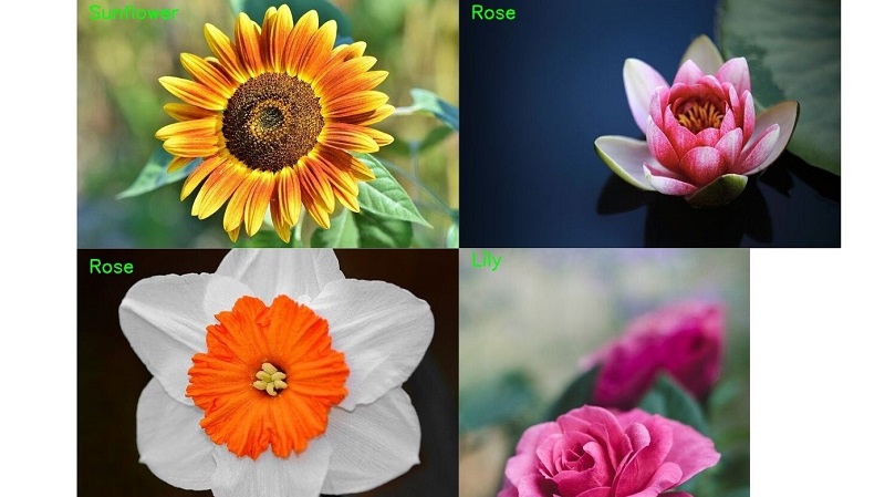
Except for the sunflower, all the other predictions are wrong. There is a reason for such poor performance as well. HOG almost always works well in those cases, where the gradient features are very definite and distinct from one another. In the case of the above flowers, the gradient features may be very similar to one another. For surety, we can take a look at the test image features.

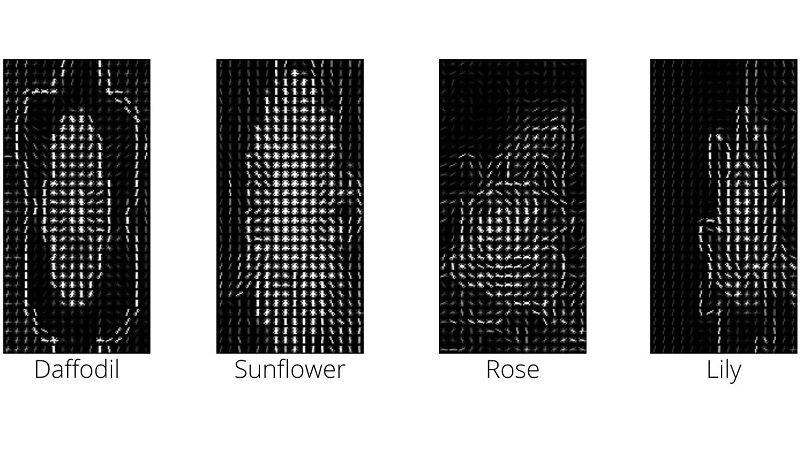
You can see how confusing the features are in the form of gradients for the sunflower and daffodil images. This is difficult even for humans to tell which image is a daffodil and which is a sunflower. Such confusing features may be the main reason for such poor predictions. Similarly, the gradients of rose and lily flowers look almost the same.

We also have the person, car, and cup dataset. Let’s see how the Linear SVM performs on that dataset.

python hog_image_recognition.py --path person_car_cup

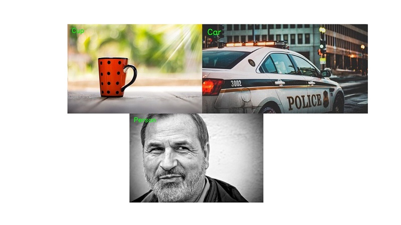
Here, the Linear SVM is predicting all three images correctly. How did this happen in this case? Maybe the HOG features will give us a better idea.

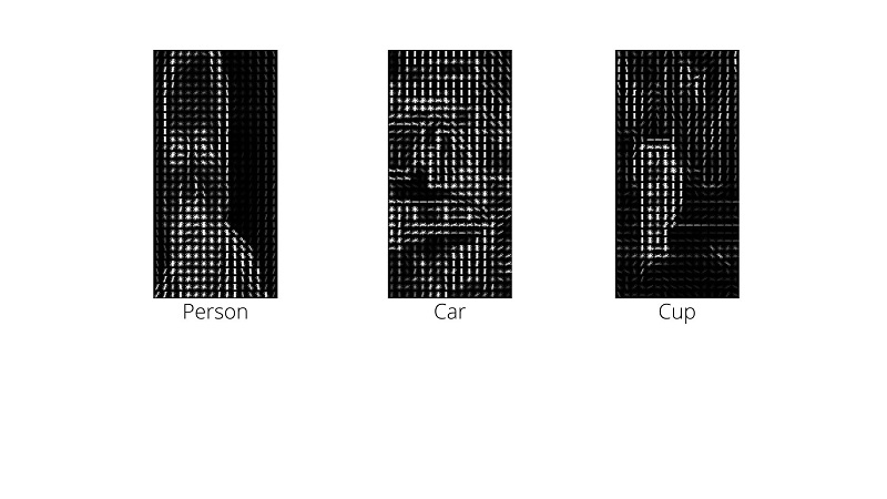
In this case, each of the features is very distinguishable from one another. We can easily tell one category from another even without the captions.

So, all in all, HOG is a great feature descriptor that we can use for image recognition. But the images that we use should have very distinguishable gradients, else the HOG feature descriptor may perform poorly.

Summary and Conclusion

In this tutorial, you learned about the HOG feature descriptor, the steps to get the HOG features from an image, and the best hyperparameters to use. You also got hands-on experience in using Histogram of Oriented Gradients for image recognition. While doing so, you got to learn the strengths and weaknesses of the HOG feature descriptor.

If you have any thoughts, doubts, or suggestions, then you can leave them in the comment section. I will surely address them.

You can contact me using the Contact section. You can also find me on LinkedIn, and Twitter.