Image Super-Resolution using Deep Learning and PyTorch

In this tutorial, you will learn how to get high-resolution images from low-resolution images using deep learning and the PyTorch framework. This post will show you how to carry out image super-resolution using deep learning and PyTorch.

In one of my previous articles, I discussed Image Deblurring using Convolutional Neural Networks and Deep Learning. We had practical experience of using deep learning and the SRCNN (Super-Resolution Convolutional Neural Network) architecture to deblur the Gaussian blurred images.

This post will take that concept a bit further. We will try to replicate the original implementation of the Image Super-Resolution Using Deep Convolutional Networks paper. We will go over the details in the next section.

Implementation Details

We will go over the implementation details of the paper and this tutorial in this section. You can find all the details about the paper and the code here.

The SRCNN Architecture

In this tutorial, we will use the same SRCNN architecture as the authors have described in their paper.

You will find more about the SRCNN architecture in this post.

The following two images compliment the SRCNN architecture.

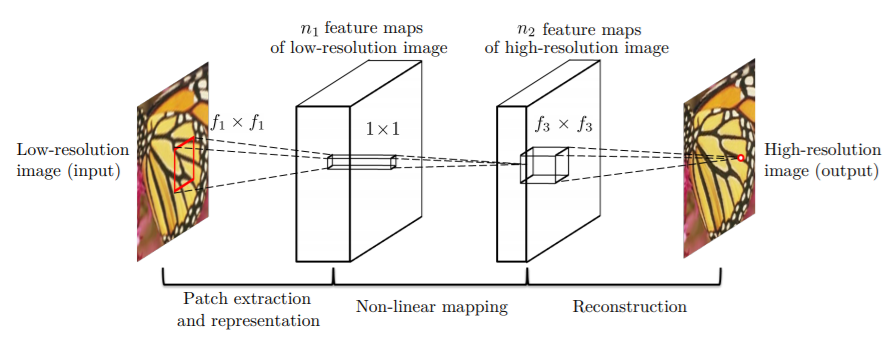
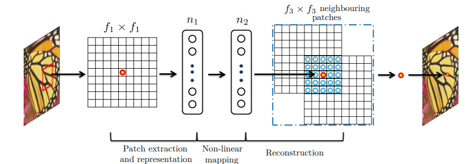
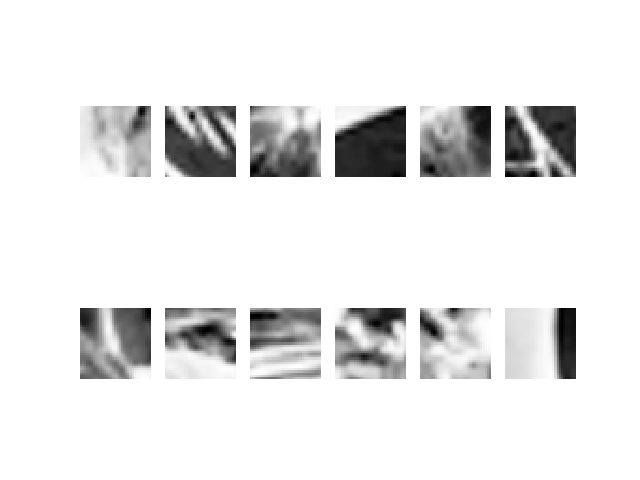
Figure 1 shows the different kernels/filters of the SRCNN architecture. You can see that there are three layers. Figure 2 shows the patch extraction process that is done by the SRCNN model.

There are three convolutional layers in the SRCNN model. We apply the ReLU activation to the first two convolutional layers only.

To get an in-depth explanation of the architecture, I recommend that you read the original paper.

Results from the SRCNN Model

The paper was released and implemented by Chao Dong, Chen Change Loy, Kaiming He, Xiaoou Tang in 2015. And at that time it surpassed the image super-resolution techniques.

In image super-resolution, we need to feed a blurry image and clean high-resolution to the neural network. The blurry image acts as the input data and the high-resolution image acts as the input label. With each iteration, the deep neural network tries to make the blurry images look more and more like the high-resolution images. The common technique to test the similarity between the two images is PSNR (Peak Signal to Noise Ratio).

The higher the PSNR, the better and more high-resolution images we get from the low-resolution images. It is calculated in dB.

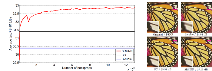
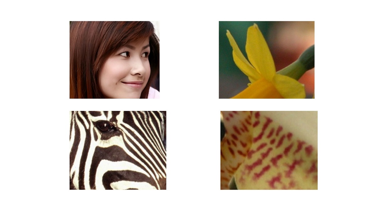
Figure 3 shows the results that the author obtained after they implemented their method and neural network on a dataset containing 91 images.

The Dataset

The authors used 91 images for training the neural network. But they did not feed those 91 images to the neural network directly. Rather they divided those images into 32×32 sub-images which correspond to 24,800 images.

You can find a whole lot of image dataset mainly used for super-resolution experimentation in this public Google Drive folder. And the dataset that we are talking about is the T91 dataset.

The authors have provided links to download the Caffe and Matlab code.

We will not write the code for generating the image patches in this tutorial. In fact, I found this GitHub repository by YapengTian which has the code to generate the image patches. The code is in MatLab and I ran it myself to generate the sub-images. These are stored as .h5 files.

Also, we will be needing some test images to test our neural network once we train it. The common datasets for testing are the Set5 and Set14 datasets. You will find those datasets in the previously mentioned Google Drive.

In this tutorial, we will test our neural network on the Set5 dataset. I will be providing the google drive link to download the image patches .h5 file and the test dataset. That will help us solely focus on the neural network architecture and coding part with PyTorch in this post.

The sub-images are stored in greyscale format. In case, you want to know how the sub-images look like, the following figure will help.

The Loss Function

We will use the same loss function as the authors. That is the MSE (Mean Square Error) loss function. Although PSNR provides the image quality estimation, still, we need something to track the improvement of our neural network. We will do this through the MSE loss function.

As per the authors, the formula for the loss function is,

$$
L(\Theta) = \frac{1}{n}\sum_{i=1}^{n}\||F(Y_i;\Theta), X_i||^2
$$

In the above formula, \(Y_i\) is the low-resolution sub-image, \(X_i\) is the high-resolution sub-image, and \(n\) is the number of training examples.

Other Code Implementations

There are a many other implementation of image super-resolution based on the same paper. Here are a few.

• SRCNN-Keras by YapengTian has the implementation using Keras API.
• SRCNN-Tensorflow by jinsuyoo has the implementation using the TensorFlow deep learning library.

But I did not find an implementation of the paper using the PyTorch framework. So, I went through the original Caffe and Matlab code and implemented the code using PyTorch. And for generating the training sub-images I used the Matlab code from SRCNN-Keras by YapengTian.

The Training and Test Data

You can download the training and test data from the google drive link below.

In the next section, we will go over the project directory structure.

The Project Structure

This is the directory structure that we will follow through this tutorial.

├───input
│   ├───bicubic_2x
│   ├───Set5
│   ├───T91
|    train_mscale.h5
├───outputs
└───src
│    srcnn.py
│    test.py
│    train.py

• The input folder contains three subfolders.
  • bicubic_2x contains the blurred bicubic images that we will use for testing. Basically, we will give the bicubic blurred images as input to the trained SRCNN neural network model. And hopefully, we will obtain a high-resolution clearer image as output.
  • Set5 folder contains the original colored test images. Be sure to take a look at those.
  • T91 contains the original colored training images. We use these RGB images to obtain the sub-images and store them as train_mscale.h5 file.
• The outputs folder will contain all our outputs while training and validating.
• src folder contains our python scripts.
  • srcnn.py contains the module for the SRCNN neural network model.
  • train.py contains the training script.
  • And test.py contains the test script that we will use after training the model.

The SRCNN Architecture Module

In this section, we will write the code to construct the SRCNN module. In the paper, the authors describe more than one SRCNN architecture. Each of them contains a different kernel size in each layer. We will use the 9 => 1 => 5 version.

The following code block defines the SRCNN neural network architecture. The code in this section goes into the srcnn.py file.

import torch.nn as nn
import torch.nn.functional as F

class SRCNN(nn.Module):
    def __init__(self):
        super(SRCNN, self).__init__()

        self.conv1 = nn.Conv2d(1, 64, kernel_size=9, padding=2, padding_mode='replicate') # padding mode same as original Caffe code
        self.conv2 = nn.Conv2d(64, 32, kernel_size=1, padding=2, padding_mode='replicate')
        self.conv3 = nn.Conv2d(32, 1, kernel_size=5, padding=2, padding_mode='replicate')

    def forward(self, x):
        x = F.relu(self.conv1(x))
        x = F.relu(self.conv2(x))
        x = self.conv3(x)

        return x

As per the original implementation, we have 64 output filters and a kernel size of 9×9 in the first convolutional layer. The second convolutional layer has 32 output filters and a kernel size of 1×1. Similarly, 1 filter (greyscale sub-images) and 5×5 kernel size for the third convolutional layer.

You can see that we use padding_mode as replicate while defining the convolutional layers. This is because, the authors also have used the same in the Caffe version of the code. I tried to keep the architecture as close to the original version as possible.

In the forward() function, we are applying ReLU activation to the first and second convolutional layers only.

In the next section, we will write the code to train the SRCNN neural network model.

Writing the Training Code for Image Super-Resolution

The code in this section will go into the train.py file.

Now, we will start writing the training code. I will explain the code wherever required. Let’s start with the imports.

import torch
import matplotlib
import matplotlib.pyplot as plt
import time
import h5py
import srcnn
import torch.optim as optim
import torch.nn as nn
import numpy as np
import math

from torch.utils.data import DataLoader, Dataset
from tqdm import tqdm
from sklearn.model_selection import train_test_split
from torchvision.utils import save_image

matplotlib.style.use('ggplot')

There are some specific imports that are not very commonly used.

• We will use the h5py module to read the train_mscale.h5 training file.
• PyTorch’s save_image module will help us easily save the images according to batch size while validating.
• Also, we import the srcnn module that contains our SRCNN architecture.

We also need to set the learning parameters for our SRCNN model. The following are the learning parameters that we will use.

# learning parameters
batch_size = 64 # batch size, reduce if facing OOM error
epochs = 100 # number of epochs to train the SRCNN model for
lr = 0.001 # the learning rate
device = 'cuda' if torch.cuda.is_available() else 'cpu'

• We will use a batch size of 64. As each sub-image is only 33×33 in dimension, a batch size of 64 should not cause Out Of Memory error.
• We will train the SRCNN mode for 100 epochs. This will not take long. The training is really fast. This is because the SRCNN deep learning model is not too big and the sub-images are small as well.
• The learning rate is 0.001.
• Finally, we set the computation device for training. Training on a GPU is going to be much faster than training on a CPU

Reading the Training Data and Preparing the Training and Validation Set

We will divide the train_mscale.h5 data into a training and validation set.

Remember that all of our sub-images are 33×33 in dimension. They are all in greyscale format. So, the number of channels is 1. Also, they are channels last from the beginning. So, we need not change that for our PyTorch SRCNN deep learning model.

Let’s start with setting the input image dimensions.

# input image dimensions
img_rows, img_cols = 33, 33
out_rows, out_cols = 33, 33

The img_rows and img_cols refer to the height and width dimension of the input sub-images. Similarly, the out_rows and out_cols refer to the height and width dimensions of the high-resolution sub-images that will act as the labels.

Now, we will read the input file and separate the training sub-images and training labels.

file = h5py.File('../input/train_mscale.h5')
# `in_train` has shape (21884, 33, 33, 1) which corresponds to
# 21884 image patches of 33 pixels height & width and 1 color channel
in_train = file['data'][:] # the training data
out_train = file['label'][:] # the training labels
file.close()

# change the values to float32
in_train = in_train.astype('float32')
out_train = out_train.astype('float32')

• On line 1, we read the train_mscale.h5 file.
• Note that it contains a total of 21884 sub-images instead of 24800 sub-images as described by the authors. This is because our data preparation style was a bit different from the original one. This should not affect the results in a big way.
• The in_train and out_train (lines 4 and 5) contain the training image data and training image labels.
• Lines 9 and 10 change the image pixel values to float32 format.

Finally, we will divide the data into training and validation set. We will use 25% of the data for validation and the rest (75%) for training.

(x_train, x_val, y_train, y_val) = train_test_split(in_train, out_train, test_size=0.25)
print('Training samples: ', x_train.shape[0])
print('Validation samples: ', x_val.shape[0])

Preparing the Custom Dataset Module and the Iterable Data Loaders

We will define our own custom dataset module using PyTorch’s Dataset class. Let’s call our dataset module as SRCNNDataset(). The following is the code for the same.

# the dataset module
class SRCNNDataset(Dataset):
    def __init__(self, image_data, labels):
        self.image_data = image_data
        self.labels = labels

    def __len__(self):
        return (len(self.image_data))

    def __getitem__(self, index):
        image = self.image_data[index]
        label = self.labels[index]
        return (
            torch.tensor(image, dtype=torch.float),
            torch.tensor(label, dtype=torch.float)
        )

• In the __init__() function we initialize the self.image_data and self.labels. Just keep in mind that in this dataset, the labels are also images. Simply, the input data are the low-resolution images and the labels are high-resolution images.
• From line 10, we define the __getitem__() function. We return both, the input data and labels as PyTorch float tensors as they are both images.

Before we define the training and validation data loaders, we need to initialize the training and validation dataset.

# train and validation data
train_data = SRCNNDataset(x_train, y_train)
val_data = SRCNNDataset(x_val, y_val)

# train and validation loaders
train_loader = DataLoader(train_data, batch_size=batch_size)
val_loader = DataLoader(val_data, batch_size=batch_size)

In the above code block, at lines 6 and 7, we define our training data loader and validation data loader as train_loader and val_loader respectively.

Initialize the SRCNN Model

Now, we will initialize our SRCNN model. We have already imported the srcnn file. Initializing it just one line of code.

# initialize the model
print('Computation device: ', device)
model = srcnn.SRCNN().to(device)
print(model)

We also load the model onto the computation device at line 3.

The authors used the Stochastic Gradient Descent (SGD) optimizer in the original implementation. With that, they obtained a PSNR of more than 32 dB. But we will use the Adam optimizer in this tutorial. I will tell the reason for the change after we obtain the results once we train the SRCNN model. Also, we will use the MSELoss as the criterion for our neural network.

# optimizer
optimizer = optim.Adam(model.parameters(), lr=lr)
# loss function 
criterion = nn.MSELoss()

Define the PSNR Function

This is probably the most important part of the tutorial. The similarity between the results we obtain and the high-resolution images is measured according to the PSNR value. The higher the PSNR value, the better.

The function that we will define here is in accordance with the original Caffe implementation by the authors. Let’s write the code first, then we will get to the explanation part.

def psnr(label, outputs, max_val=1.):
    """
    Compute Peak Signal to Noise Ratio (the higher the better).
    PSNR = 20 * log10(MAXp) - 10 * log10(MSE).
    https://en.wikipedia.org/wiki/Peak_signal-to-noise_ratio#Definition
    First we need to convert torch tensors to NumPy operable.
    """
    label = label.cpu().detach().numpy()
    outputs = outputs.cpu().detach().numpy()
    img_diff = outputs - label
    rmse = math.sqrt(np.mean((img_diff) ** 2))
    if rmse == 0:
        return 100
    else:
        PSNR = 20 * math.log10(max_val / rmse)
        return PSNR

If you need to learn more about PSNR, then you can click on the link in the comments in the above code block.

The psnr() function takes in three parameters. The first one is the original label from the data. The second one is the outputs that we obtain after feeding the low-resolution sub-images to the SRCNN model. And the third one has a default value of 1 (max_val) . The max_val parameter is the maximum value of the pixel in our data. As we have all the pixels in our data in-between 0 and 1, therefore, the max_val is also 1.

At lines 8 and 9, we load the label and outputs on to the CPU and convert them into NumPy vectors. We need to do this before doing any mathematical and NumPy operations on the values. We cannot do those operations on the torch tensors when they have requires_grad as True.

Line 10, calculates the difference (img_diff) between the outputs and original label. Then at line 11, we find the RMSE (Root Mean Square Error) using the calculated img_diff.

If the RMSE is 0, then we return 100. Else, we calculate the PNSR using the max_val and rmse at line 16. Finally, we return the PSNR value.

The Training Function

In this section, we will define our training function. We will call it train.

The following is the train() function definition.

def train(model, dataloader):
    model.train()
    running_loss = 0.0
    running_psnr = 0.0
    for bi, data in tqdm(enumerate(dataloader), total=int(len(train_data)/dataloader.batch_size)):
        image_data = data[0].to(device)
        label = data[1].to(device)
        
        # zero grad the optimizer
        optimizer.zero_grad()
        outputs = model(image_data)
        loss = criterion(outputs, label)

        # backpropagation
        loss.backward()
        # update the parameters
        optimizer.step()

        # add loss of each item (total items in a batch = batch size)
        running_loss += loss.item()
        # calculate batch psnr (once every `batch_size` iterations)
        batch_psnr =  psnr(label, outputs)
        running_psnr += batch_psnr

    final_loss = running_loss/len(dataloader.dataset)
    final_psnr = running_psnr/int(len(train_data)/dataloader.batch_size)
    return final_loss, final_psnr

The above train() function is like any other training function in PyTorch except with a few changes.

• We define two variables, running_loss and running_psnr to keep track of the batch-wise loss and PSNR values.
• As usual, we are zeroing out the optimizer, backpropagating the gradients, and updating the parameters.
• The important thing to note here are lines 22 and 23. At line 22, we get the batch_psnr value by calling the psnr() function. Then at line 23, we add the batch_psnr to the running_psnr.
• Now, remember that psnr is not an in-built PyTorch function. So, it does have a .item() attribute. That means we get the PSNR value for the whole batch. That’s why at line 26, we get the epoch-wise PNSR value (final_psnr) by dividing the running_psnr by the number of batches.

The Validation Function

Here, we will define the validation function, we will call it validate().

def validate(model, dataloader, epoch):
    model.eval()
    running_loss = 0.0
    running_psnr = 0.0
    with torch.no_grad():
        for bi, data in tqdm(enumerate(dataloader), total=int(len(val_data)/dataloader.batch_size)):
            image_data = data[0].to(device)
            label = data[1].to(device)
            
            outputs = model(image_data)
            loss = criterion(outputs, label)

            # add loss of each item (total items in a batch = batch size) 
            running_loss += loss.item()
            # calculate batch psnr (once every `batch_size` iterations)
            batch_psnr = psnr(label, outputs)
            running_psnr += batch_psnr
        outputs = outputs.cpu()
        save_image(outputs, f"../outputs/val_sr{epoch}.png")

    final_loss = running_loss/len(dataloader.dataset)
    final_psnr = running_psnr/int(len(val_data)/dataloader.batch_size)
    return final_loss, final_psnr

The validate() function is accepting an extra epoch parameter. We will use this to save the sub-images after each epoch. From that we will be able to know whether the sub-images are really getting near to high-resolution or not.

We need not backpropagate the gradients or update the parameters while validating. We are using the save_image() function to save the sub-images after each validation epoch to the disk.

Running the train() and validate() Funtions

We will train and validate the SRCNN model for 100 epochs as defined before. The following block of code does that for us.

train_loss, val_loss = [], []
train_psnr, val_psnr = [], []
start = time.time()
for epoch in range(epochs):
    print(f"Epoch {epoch + 1} of {epochs}")
    train_epoch_loss, train_epoch_psnr = train(model, train_loader)
    val_epoch_loss, val_epoch_psnr = validate(model, val_loader, epoch)
    print(f"Train PSNR: {train_epoch_psnr:.3f}")
    print(f"Val PSNR: {val_epoch_psnr:.3f}")
    train_loss.append(train_epoch_loss)
    train_psnr.append(train_epoch_psnr)
    val_loss.append(val_epoch_loss)
    val_psnr.append(val_epoch_psnr)
end = time.time()
print(f"Finished training in: {((end-start)/60):.3f} minutes")

We have four lists in the above code block. The train_loss, val_loss lists will store the loss values after each epoch, The train_psnr and val_psnr will store the PSNR values after each epoch.

Then we execute the train() and validate() functions inside a for loop for 100 epochs.

Finally, we print the training time at line 15.

Saving the Graphical Plots and the Model

Now, we just need to save the graphical plots for the loss and PSNR values so that we can analyze them later. We will also save the model weights to disk. This is so that we can load them and easily test the model on our test data.

# loss plots
plt.figure(figsize=(10, 7))
plt.plot(train_loss, color='orange', label='train loss')
plt.plot(val_loss, color='red', label='validataion loss')
plt.xlabel('Epochs')
plt.ylabel('Loss')
plt.legend()
plt.savefig('../outputs/loss.png')
plt.show()

# psnr plots
plt.figure(figsize=(10, 7))
plt.plot(train_psnr, color='green', label='train PSNR dB')
plt.plot(val_psnr, color='blue', label='validataion PSNR dB')
plt.xlabel('Epochs')
plt.ylabel('PSNR (dB)')
plt.legend()
plt.savefig('../outputs/psnr.png')
plt.show()

# save the model to disk
print('Saving model...')
torch.save(model.state_dict(), '../outputs/model.pth')

Execute the train.py File

Run the train.py file while being within the src folder in the terminal.

python train.py

The following is the truncated output that we get while training the SRCNN deep learning model.

Epoch 1 of 100
256it [00:12, 19.84it/s]
34%|█████████████████████▉                                           | 86/255 [00:01<00:03, 55.92it/s]
Train PSNR: 22.638
Val PSNR: 8.720
Epoch 2 of 100
256it [00:08, 28.52it/s]
 34%|█████████████████████▉                                           | 86/255 [00:01<00:03, 55.17it/s]
Train PSNR: 26.470
Val PSNR: 9.096
...
Epoch 100 of 100
256it [00:08, 29.25it/s]
 34%|█████████████████████▉                                           | 86/255 [00:01<00:02, 58.62it/s]
Train PSNR: 28.631
Val PSNR: 9.674
...
Saving model...

By the end of the training, we are getting a training PSNR value of 28.631 dB. This is lower than the 32 dB that the author obtained in their original implementation. Let’s analyze the PSNR plot that we have saved to the disk.

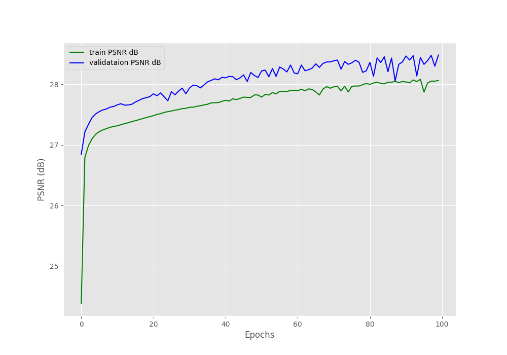
You can see that there is a large gap between the training PSNR plot and the validation PSNR plot. The validation PSNR value is only 9.67 dB by the end of the training. This large variance can be due to the split percentage of our training and validation data or maybe because of using Adam optimizer instead of SGD. Let’s hope that it does not affect the test results that much.

Testing the Trained SRCNN Model

In this section, we will write the code to test our trained SRCNN deep learning model. We will test the low-resolution bicubic images that are inside input/bicubic_2x folder.

Also, we will have to convert images to greyscale first. This is because the neural network model is also trained on greyscale images.

All the code from here on will go into the test.py file.

The following are the imports that we will need along the way.

import torch
import cv2
import srcnn
import numpy as np
import glob as glob
import os

from torchvision.utils import save_image

Now, let’s set the computation device.

device = 'cuda' if torch.cuda.is_available() else 'cpu'

Note: If you have trained your model on the CPU, then you have to explicitly use CPU while testing as well.

Next, we will initialize the model and load the trained model weights.

model = srcnn.SRCNN().to(device)
model.load_state_dict(torch.load('../outputs/model.pth'))

Giving the Test Images as Input to the Trained Model

You can see that we have only 5 images for testing. As this a very small number, we can give the all images for testing inside a for loop to the model. This should not take much time considering the small number of images.

image_paths = glob.glob('../input/bicubic_2x/*')
for image_path in image_paths:
    image = cv2.imread(image_path, cv2.IMREAD_COLOR)
    test_image_name = image_path.split(os.path.sep)[-1].split('.')[0]

    image = cv2.cvtColor(image, cv2.COLOR_BGR2GRAY)
    image = image.reshape(image.shape[0], image.shape[1], 1)
    cv2.imwrite(f"../outputs/test_{test_image_name}.png", image)
    image = image / 255. # normalize the pixel values
    cv2.imshow('Greyscale image', image)
    cv2.waitKey(0)


    model.eval()
    with torch.no_grad():
        image = np.transpose(image, (2, 0, 1)).astype(np.float32)
        image = torch.tensor(image, dtype=torch.float).to(device)
        image = image.unsqueeze(0)
        outputs = model(image)

    outputs = outputs.cpu()
    save_image(outputs, f"../outputs/output_{test_image_name}.png")
    outputs = outputs.detach().numpy()
    outputs = outputs.reshape(outputs.shape[2], outputs.shape[3], outputs.shape[1])
    print(outputs.shape)
    cv2.imshow('Output', outputs)
    cv2.waitKey(0)

• At line 1, we get all the image paths using the glob module.
• Then we use a for loop to test on each of the 5 images. We read the image at line 3.
• At line 4, we get just the image name so that we can easily save the original test image and the output image to the disk.
• We convert the image to greyscale format at line 6 and make it channels-last so as to visualize it using OpenCV.
• At line 9, we divide the pixel values by 255 so that all values are within 0 and 1 now.
• Then we show the original test image.
• At line 14, we switch to eval mode. Line 16 makes the image channels-first and line 17 converts it into a torch tensor. Then we unsqueeze it to add an extra batch dimension.
• Line 19 feeds the image to the model and we get the output.
• From lines 21 to 27, we save the output image to disk, make it channels-first again, and finally visualize it using OpenCV.

Executing the test.py Script

We are all set to execute the test.py script. Remember that all the five images will be run through the model in the same execution cycle. So, be ready to press the q key a lot of time.

While being within the src folder in the terminal, you just need to type the following command.

python test.py

Let’s visualize the outputs that we are getting.

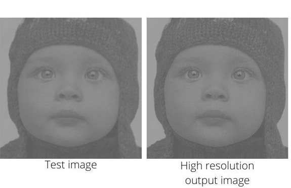
Figure 7 shows the test image that we give as input on the left. And the right side image is the high-resolution output that the model produces. Although the results are not magically good, still the output looks much sharper and clearer than the one the left. I think that the results are good enough for starting out.

Let’s check out the other outputs.

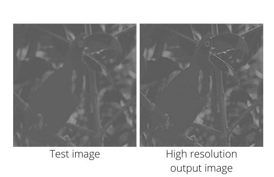
In Figure 8 we can see that the output image looks a bit too sharp at the edges of the beak of the bird. The results look a bit out of place to be realistic. Looks like we found one limitation of the SRCNN model. It can sometimes over-sharp the images.

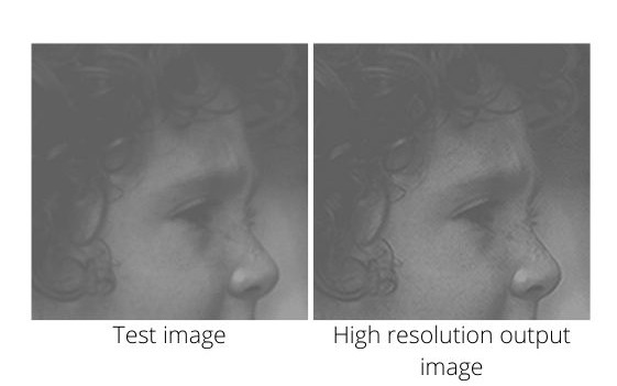
Figure 9 shows the head of a girl. We can see that the output image shows sharper and clearer hair and eye lines. This time the results are pretty good.

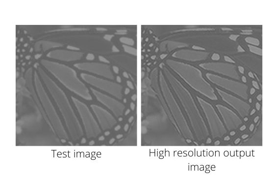
The butterfly wing in Figure 10 is perhaps one of the best outputs that we got. The patterns in the wing are very clear in the output image. Even the edges look good in the output image.

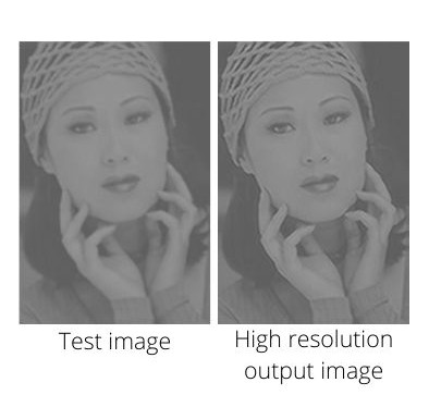
Finally, Figure 11 really shows how good our SRCNN deep learning model is. The differences between the test image and the high-resolution input image are striking. The patterns of the head band of the woman are particularly sharp in the output image. Also, her eyebrows, eyes, and fingers are very clear and sharp.

Looks like our model has learned well enough to turn low-resolution images to high-resolution images. But you can improve the SRCNN model a lot.

Further Improvements and Changes

Although our SRCNN deep learning model is performing well enough, we can still improve further. The following points will help you.

• The authors used the SGD optimizer instead of Adam optimizer. Along with that, they also used different learning rates for different layers. The learning rate was 0.0001 for the first two convolutional layers and 0.00001 for the last convolutional layer. But we only used a learning rate of 0.001 for all layers.
• The authors trained their model for 8×10\(^8\) backpropagations. But we trained our SRCNN model for only 100 epochs. You can try and train the model for longer.
• You can try and extend the project for training and testing on color images.

Along with the above points, the following research papers might help you a lot in moving the further.

• Image super-resolution as sparse representation of raw image patches, Jianchao Yang, John Wright, Yi Ma, Thomas Huang.
• Image Deblurring with BlurredNoisy Image Pairs, Lu Yuan, Jian Sun, Long Quan, Heung-Yeung Shum.

Also, the following GitHub repositories will help you understand a lot of internal code and data preparation processes.

• Basic Super-Resolution Toolbox, including SRResNet, SRGAN, ESRGAN, etc.
• TensorFlow implementation of SRCNN.

Summary and Conclusion

In this tutorial, you learned how to carry out image super-resolution using the SRCNN deep learning model. You got to implement the SRCNN model architecture and train it on sub-images to get the results. You also learned what the authors of the paper did differently and ways to improve the model further.

I hope that you learned a lot from this tutorial. If you have any doubts, thoughts, or advice, please feel free to use the comment section. I will surely address them.

You can contact me using the Contact section. You can also find me on LinkedIn, and Twitter.