
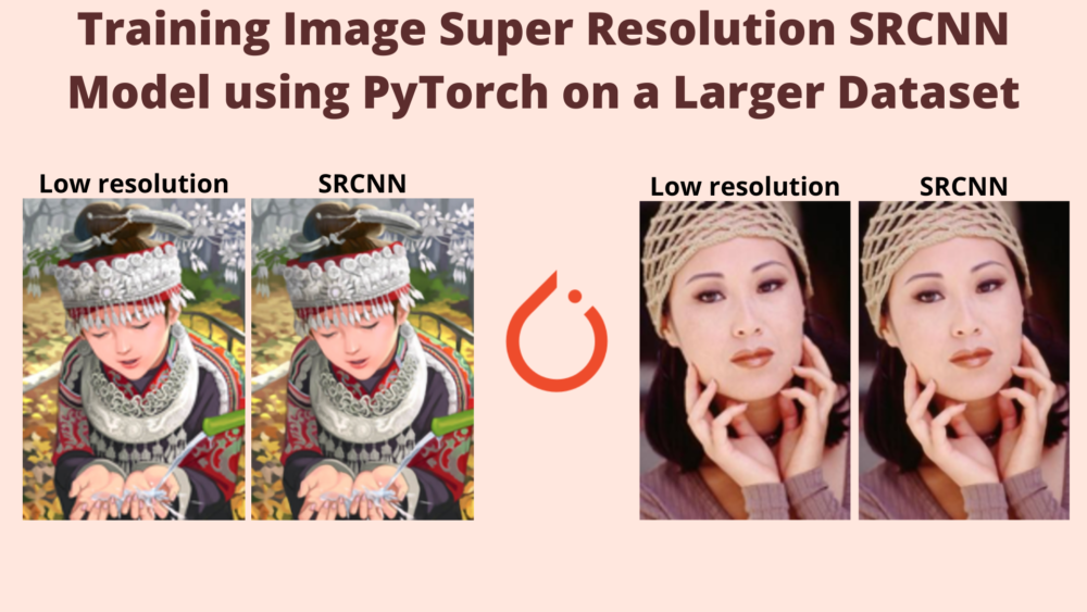
In this tutorial, we will be training the image super resolution model, that is SRCNN using the PyTorch deep learning framework. In the previous post, we implemented the original SRCNN model on the T91 dataset which was introduced in this paper. This tutorial takes the previous implementation a step further. We will train a larger model on an even larger dataset. This model was also discussed in the paper. Along with that, we will combine the T91 dataset with another image super image dataset, which is the General100 dataset. We will discuss all the details in one of the further sections.
I have already covered the concept and basic code of image super resolution using SRCNN and PyTorch in one of the previous tutorials. But that tutorial had its limitations which we will discuss shortly.
Before we get into the details of the post, let’s check out the topics that we will cover here.
- Why do we need to cover this post and why learn about image super resolution?
- The SRCNN architecture for image super resolution using PyTorch.
- Training the SRCNN model on the T91 and General100 datasets.
- Testing the SRCNN model on the Set14 and Set5 images.
This is the second post in the SRCNN with PyTorch series.
- Image Super Resolution Using Deep Convolutional Networks: Paper Explanation
- SRCNN Implementation in PyTorch for Image Super Resolution
- Image Super Resolution using SRCNN and PyTorch – Training a Larger Model on a Larger Dataset
Posts To Read If You are New to Image Super Resolution
If you are completely new to the topic of image super resolution and the SRCNN architecture, then it’s better to read a few of the previous posts.
- Image Super Resolution Using Deep Convolutional Networks: Paper Explanation – In this post, we discuss the original SRCNN paper. This will give you a good overview of the SRCNN architecture, the datasets, the implementation, and the results.
- SRCNN Implementation in PyTorch for Image Super Resolution – In this post, we implement the original baseline SRCNN architecture from the paper. Not only that, we train it on the T91 dataset and test it on the Set5 and Set14 datasets as well. This is will be a good starting point to get into the coding part of image super resolution.
Let’s jump into the post now.
Why This Post and Why Learn About Image Super Resolution?
First, let’s check out why we need this post.
I had already written another post on image super resolution using the SRCNN model before. But it had a few limitations which can add up quickly when trying to scale to larger datasets and models. Let’s check out what the limitations were in the older post:
- First of all, the model was trained on grayscale images and not on colored (RGB) images. This means that we could only run inference on grayscale images.
- In that post, we converted the training dataset into
.h5format using Matlab code. This means that the training and validation datasets were entirely loaded into memory before training. This poses a huge limitation when dealing with larger datasets and models. We need to be able to load the images in batches so that we can use as large a dataset as we want.
Apart from that, in the previous post, we implemented the original SRCNN model as well. Although we trained it on the T91 dataset and tested it on the Set5 and Set14 datasets, we still can do much better. Which is combining the T91 and General100 datasets for training. We will combine that with one of the larger models from the paper which is bound to give us better results.
I hope that you are now interested to follow along with this tutorial.
The SRCNN Architecture for Image Super Resolution
In this post, we use the SRCNN architecture from the paper Image Super-Resolution Using Deep Convolutional Networks by Dong et al.
Now, we have covered the SRCNN architecture in detail in the previous few posts. You can find all the details here:
- Paper Explanation: Image Super Resolution Using Deep Convolutional Networks
- Image Deblurring using Convolutional Neural Networks and Deep Learning
- Image Super-Resolution using Deep Learning and PyTorch
In the final post from the above list, you will also find details about the loss functions and the PSNR metric which are not going to change in this tutorial. If you are new to the topic, having a look at them may also help.
Here, we will cover the architecture in brief and mostly focus on our own implementation details.
The SRCNN Model
Let’s go through a few general details of the SRCNN model first.
The SRCNN model is a simple fully convolutional neural network.

Figure 2 shows the general architecture and implementation of the SRCNN model. We give a low resolution image \(Y\) as input to the image. The model layers try to map this low resolution image to a high resolution target image, \(X\). The model produces the final high resolution images by passing the low resolution images through a series of non-linear functions. We can write:
$$
X = F(Y)
$$
In the above figure, \(n_1\) and \(n_2\) represent the number of output channels of the convolutional layers. On a similar note, \(f_x\) x \(f_x\) represent the kernel sizes of the convolutional layers.
There are a few different implementations of the SRCNN model according to which the number of output channels and kernel sizes change. In this tutorial, we will use the most general architecture. We will explore more about the practical aspects of the model in the next section.
The Implementation Details
In this section, we will go through the implementation details of:
- The SRCNN model.
- The training dataset.
- The test dataset.
Implementation Details of the SRCNN Model
We will use the the larger SRCNN model from the paper which had more convolutional filters. In the model:
- \(n_1\) = 128
- \(n_2\) = 64
- \(f_1\)x\(f_1\) = 9×9
- \(f_2\)x\(f_2\) = 1×1
- \(f_3\)x\(f_3\) = 5×5
As you may observe, this model contains 128 and 64 output filters respectively. In the smaller baseline model, they were 64 and 32. Apart from that, we keep the filter sizes for the convolutional layers the same as per the approach from the paper.
The Training Datasets
We will use the T91 and General100 datasets for training the SRCNN model in this tutorial. They are the usual benchmark datasets used in many of the image super resolution papers.
In fact, we will be taking sub-images (or patches) of size 32×32 with a stride of 14 from both these datasets. We will create and store the original high resolution patches in one folder and the 2x bicubic low resolution patches in another folder. Going through the code will help you get into the details. For now, we can just keep in mind that there be more than 100000 sub-images from both of these datasets. This will allow us to train a much better model.
For example, take a look at the following figure. It shows an image of a leaf on the right from the T91 dataset. And on the left are the 32×32 patches with a stride of 14 that we generate for training.
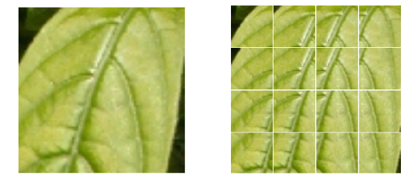
As you may observe, a few patches are overlapping because the stride is 14. Still, each patch will contain enough new features. Now, we need to keep in mind that we will be doing this for every image in the General100 and T91 datasets. So, this will give us a lot of patches. The corresponding low resolution 2x bicubic images will also be created for each patch and saved to disk. The implementation in the coding section will make things clearer.
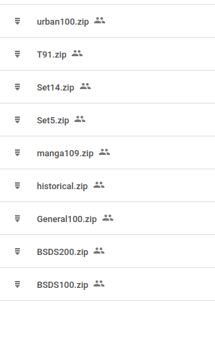
This repository by xinntao provides almost all the super resolution datasets in this Google Drive folder.
The approach that we follow here is exactly the same as in the previous post. The only difference is that we combine two datasets for training here.
The Test Dataset
For testing, we will use the same Set14 and Set5 datasets that you can find in the same Google Drive folder.
You may either download the dataset from there, or you will also get access to the datasets when downloading the zip file for this tutorial.
Directory Structure
For now, let’s get familiar with the directory structure of this tutorial.
├── input
│   ├── General100
│   ├── Set14
│   ├── Set5
│   ├── T91
│   ├── test_bicubic_rgb_2x
│   ├── test_hr
│   ├── train_hr_patches
│   ├── train_lr_patches
│   ├── General100.zip
│   ├── Set14.zip
│   ├── Set5.zip
│   └── T91.zip
├── outputs
│   ├── valid_results
│   ├── loss.png
│   ├── model_ckpt.pth
│   ├── model.pth
│   └── psnr.png
├── src
│   ├── bicubic.py
│   ├── datasets.py
│   ├── patchify_image.py
│   ├── srcnn.py
│   ├── test.py
│   ├── train.py
│   └── utils.py
└── NOTES.md
The above directory structure is almost the same as we had in the last post with only a few minor differences. Let’s list out the changes.
- As we are combining the T91 and General100 dataset this time, we call the training images (low resolution images) directory as
train_lr_patches. And we call the labels (high resolution images) directory. astrain_hr_patches. They are all present in theinputdirectory where the new General100 dataset is also present.
For now, you may download the zip file for this tutorial. Extracting it will already provide every directory and file in the proper format. You can right away run the training or testing, whichever you may wish.
Libraries and Dependencies
The following are the major libraries that we need to run the code in this tutorial.
- torch 1.11.0 and torchvision 0.12.0: You can install them according to your configuration from the official website. Other older and even newer versions of PyTorch may also work without issues.
- patchify: We need to create patchces out of images. Instead of writing a custom script, we will use this library which will make things easier for us.
Image Super Resolution using SRCNN and PyTorch
In this tutorial, we will not discuss the Python code in detail. You can find all of the major details in the previous post. The code here is almost the same apart from path changes according to the new General100 dataset.
Before starting the training, we will discuss the steps to each of the scripts sequentially to prepare the data. Then we will focus entirely on analyzing the training results, and the test results. We will also analyze whether we were able to achieve higher test PSNR this time or not.
We need the following Python files for the training part of the SRCNN model.
utils.pypatchify_image.pybicubic.pydatasets.pysrcnn.pytrain.py
After training, we will use the test.py script to test the trained SRCNN model on the Set5 and Set14 datasets.
Note that all the Python files will remain in the src directory. Also, all the training and testing took place on a machine with an i7 10th generation CPU, 10 GB RTX 3080, and 32 GB of RAM.
Let’s discuss the steps to prepare the datasets and start the training.
Creating High and Low Resolution Image Patches for Image Super Resolution using SRCNN and PyTorch
First, we need to create the 32×32 patches out of the General100 and T91 datasets.
The code to create the patches will go into the patchify_image.py script.
Open the terminal/command line inside the src directory and execute the following script.
python patchify_image.py
You should see an output similar to the following.
Creating patches for 191 images
100%|█████████████████████████████████████████| 191/191 [00:16<00:00, 11.50it/s]
After that, you will find over 100000 image patches in the train_hr_patches and train_lr_patches directories inside input.
Prepare the Set5 and Set14 Validation Images
Next, we will create the high and low resolution images for the Set5 and Set14 images. We will use these in the validation loop while training the SRCNN model.
Execute the following command from the src directory.
python bicubic.py --path ../input/Set14/original ../input/Set5/original --scale-factor 2x
The output should be similar to the following.
19
Scaling factor: 2x
Low resolution images save path: ../input/test_bicubic_rgb_2x
Original image dimensions: 250, 361
Original image dimensions: 512, 512
...
Original image dimensions: 288, 288
The validation set contains 19 images in total.
Execute train.py to Start the Training
As the dataset is ready, we are all set to run the training now. We will train the SRCNN model for 1000 epochs. In the previous post, we trained it for 2500 epochs as the dataset was small, and the SRCNN model was also the base one. As we have a larger model here and much more image patches, so we will train it for less number of epochs.
Execute the following command while being within the src directory.
python train.py --epochs 1000
The following is the truncated output from the terminal.
Computation device:  cuda
SRCNN(
  (conv1): Conv2d(3, 128, kernel_size=(9, 9), stride=(1, 1), padding=(2, 2))
  (conv2): Conv2d(128, 64, kernel_size=(1, 1), stride=(1, 1), padding=(2, 2))
  (conv3): Conv2d(64, 3, kernel_size=(5, 5), stride=(1, 1), padding=(2, 2))
)
Training samples: 104841
Validation samples: 19
Epoch 1 of 1000
100%|██████████████████████████████████████████████████████████████████| 820/820 [01:09<00:00, 11.74it/s]
100%|████████████████████████████████████████████████████████████████████| 19/19 [00:00<00:00, 58.61it/s]
Train PSNR: 24.192
Val PSNR: 27.906
Saving model...
.
.
.
Epoch 1000 of 1000
100%|██████████████████████████████████████████████████████████████████| 820/820 [00:30<00:00, 27.33it/s]
100%|████████████████████████████████████████████████████████████████████| 19/19 [00:01<00:00, 14.95it/s]
Train PSNR: 30.754
Val PSNR: 29.741
Saving model...
Finished training in: 510.745 minutes
The training took a little over 8 hours on an RTX 3080 GPU.
By the end of 1000 epochs, we have validation PSNR above 29.7. This is higher than what we had in the previous case with the smaller model and T91 dataset for training only.
Let’s take a look at the graphs.
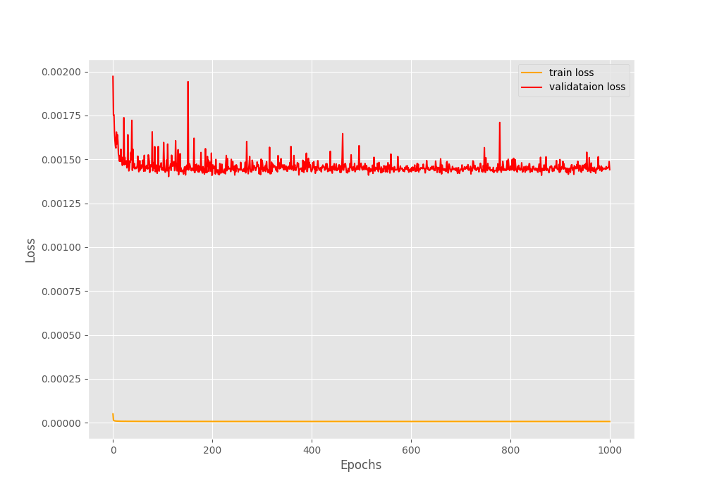
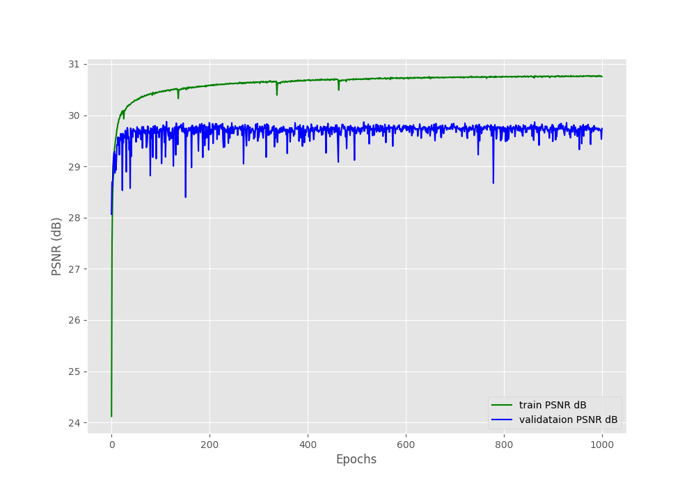
The loss graph here is almost similar to the previous training where the training loss is much lower than the validation loss. On the other hand, there seems to be a bigger gap between the training and validation PSNR this time. Nonetheless, both seem to be improving till the end of training. And almost certainly, training for longer will improve the results.
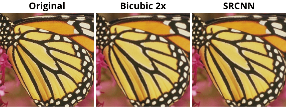
Comparing the Validation Reconstruction Images
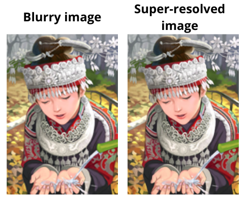
Now, let’s compare the same validation reconstruction images that we did in the previous post. This will give us a good idea of how whether we were able to train a better model or not.
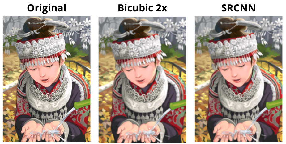
Surely, the SRCNN reconstruction looks much better compared to the bicubic upsampling. And if you observe closely, it is slightly sharper compared to the previous results in the last post.
Here, the improvements are quite visible and also look sharper compared to previous results.
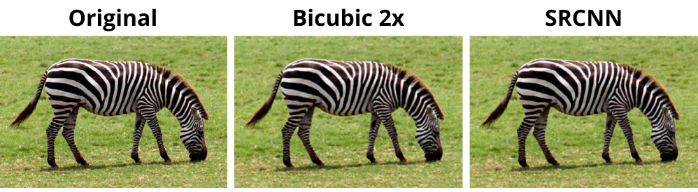
If you go through the previous post, you will notice that the reconstruction of the zebra image was not that better. But this time, the SRCNN output is much cleaner and sharper.
Testing on Set5 and Set14 Datasets
Finally, we will run the testing on the Set5 and Set14 datasets. You will find the code for it in the test.py script.
Let’s execute the script from the terminal while being within the src directory.
python test.py
The following are the test PSNR values.
100%|██████████████████████████████████████████████████████████████████████| 5/5 [00:00<00:00, 58.92it/s]
Test PSNR on Set5: 32.519
100%|████████████████████████████████████████████████████████████████████| 14/14 [00:00<00:00, 55.08it/s]
Test PSNR on Set14: 28.749
This time we got slightly higher PSNR compared to the previous training. And interestingly, we trained for less number of epochs this time. This shows how much further we can improve the results if we have more data and slightly better model.
But do note that still this is much lower than what the authors achieved with their baseline model in the original training where they trained the model for 3 days. Obviously, that was because they trained for 8×10\(^8\) iterations. Still, we did good and achieved our objective of getting better results than our previous experiment.
Summary and Conclusion
In this post, we trained the SRCNN Image Super Resolution model using the PyTorch deep learning framework. This time, we used a larger dataset and a better model. By the end of our experiments, we were able to get better results compared to one of previous training where we used a smaller dataset and a smaller model. So, all in all, it was a successful experiment. Hopefully, you learned something valuable from it as well.
If you have any doubts, thoughts, or suggestions, please leave them in the comment section. I will surely address them.
You can contact me using the Contact section. You can also find me on LinkedIn, and X.
