
For the past few years, convolutional neural networks are able to show remarkable performance in many computer vision tasks. Starting from image classification, object detection, and image segmentation, to generative models. Deep learning and convolutional neural networks are a part of all of them. There is yet another application of computer vision that has been influenced by deep convolutional neural networks. That is image super resolution. In simple words, it is obtaining high resolution images from low-resolution images. In this post, we will be discussing a very important paper on image super resolution. That is, Image Super Resolution Using Deep Convolutional Networks by Dong et al.
This was one of the first papers which explored deep convolutional neural networks for image super resolution. There have been many works after this. In this post, we will explore this paper along with their contributions, networks architecture, and experiment results. And in the next few tutorials, we will implement the paper in PyTorch according to the original experiments and with a few variations as well.
We will cover the following topics in this post:
- A short overview of image super resolution.
- Contributions of the Image Super Resolution using Deep Convolutional Networks paper.
- The approach used by the authors for image super resolution.
- Then, we will cover network architecture in detail.
- Next is the training pipeline with all the hardware and hyperparameter details.
- Finally, the experiments and the results.
This is going to be a very interesting post and we will cover as many details as possible here.
What is Image Super Resolution?
Image super resolution is the task of obtaining high resolution images from low resolution images. In terms of deep learning and computer vision, the low resolution (LR) image is the input feature. Then we train our super resolution neural network to learn the features of the low resolution input image and map it to the features of a high resolution (HR) image (which is the label).

The above image shows the process of image super resolution in a very simple manner. Although, it is better to keep in mind that there are a lot of intermediate steps involved. We will be going through almost all of them in this tutorial.
The important question is “why is image super resolution using deep learning such a big deal?”. And “why do we need image super resolution?”
See, in image super resolution, it is not necessary to obtain the high resolution images dynamically at the time of capture. Instead, we have a low resolution image, then we pass it through a neural network (at least during inference), and generate the high resolution image. This means that we have the capacity to create a better image from an already available low resolution image. In other words, we can do this in the post-processing stage rather than the time when the actual image is captured. This obviously leads to a lot of flexibility. But of course, we can make the inference pipeline a lot more dynamic to create high resolution images from video frames as they are being captured in real-time.
Why Do We Need Image Super Resolution?
Let’s check out why we need image super resolution and what we can use it for.
- The first thing that comes to mind is increasing the clarity of an image that is blurry. But this in itself can fall under any circumstances.
- For example, making photos taken by smartphones clearer can be one of the potential applications.
- In surveillance, there are a lot of situations where authorities need to clear up an image or video sequence.
- And we can also create many interesting applications using image super resolution and can deploy them as a web app for others to use.
The above cover only a few of the applications of image super resolution. There are many other interesting applications in terms of deep learning we can code through. If possible, we will cover many of them in future blog posts.
Contributions of the Image Super Resolution using Deep Convolutional Networks Paper
The very first version of the Image Super Resolution using Deep Convolutional Networks Paper by Dong et al. was released in 2014. But we will discuss the most updated version of the paper from 2015 which includes all the updates and improvements.
In the paper, the authors introduce the SRCNN architecture, that is, Super Resolution Convolutional Neural Network.
There are three important contributions:
- The SRCNN architecture is a fully-convolutional deep learning architecture. It learns to map the low resolution images to the high resolution ones with little pre or post processing.
- The paper also establishes a relationship between the deep learning super resolution method and the traditional sparse-coding based methods.
- It also shows that deep learning and computer vision can be useful for traditional computer vision problems like image super resolution. Not only that, but it is also worthwhile to note that the architecture can give real-time results during inference.
In the rest of the post, we will uncover more details about the above points and explore the architecture, the training pipeline, and also the results & experiments.
Approach Used by the Authors for Image Super Resolution using Convolutional Neural Networks
The main aim here is to obtain a high resolution image from a low resolution image.
Suppose that we have a low resolution image \(Y\) which we upscale to the desired size using bicubic interpolation. At this stage, the image is blurry because of the upscaling. Now, we want to obtain the high resolution counterpart of the same image, \(X\), which is the ground truth. We can also call \(X\) as \(F(Y)\) and we need to learn the mapping \(F\).
According to the authors, this requires three operations:
- Patch extraction and representation: This is the process of extracting overlapping patches from the low-resolution images. We will feed these as features to the SRCNN model and the corresponding high resolution patches will act as the ground truth labels.
- Non-linear mapping: The model will learn the mapping in the training phase. That is, it will learn to map the low resolution patches to the high resolution patches.
- Reconstruction: This is the final operation where the model reconstructs (or outputs) the possible high resolution image.
Patch Extraction from Images
Now, there are some important aspects regarding the overlapping patch extraction from the images. We can extract the patches from each image as a preprocessing stage and store them on a disk beforehand. For example, take the case of the very general T91 dataset for image super resolution. This is also one of the benchmark datasets in the paper.
The authors train one of the SRCNN variants by extracting 32×32 dimensional patches with a stride of 14. This resulted in 24,800 sub-images (or patches). The following is an example of an image and its patches.
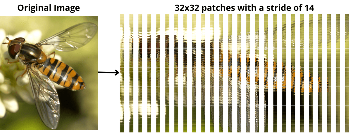
The above figure shows an image of a bee and its overlapping 32×32 dimensional patches with a stride of 14. In a future tutorial, when training the SRCNN model, we will be creating similar patches for all images.
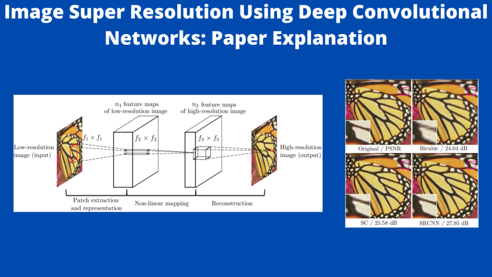
The SRCNN Architecture
To get to know the SRCNN architecture in detail, let’s directly take a look at a diagram. Then we will formulate our explanation from there.
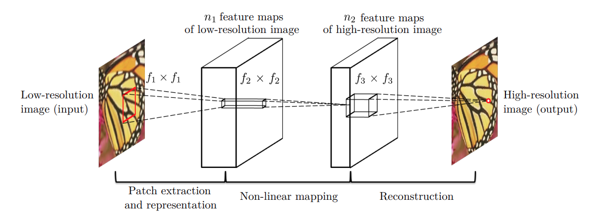
The above figure shows the general architecture of the SRCNN model. It also shows the kernel sizes (\(f_x\)x\(f_x\)) and filters (\(n_1\) and \(n_2\)) for the different convolutional layers.
We can see that the model takes a low resolution image patch, \(Y\), and outputs a high resolution image, \(F(Y)\).
There are a few different implementations of the SRCNN model according to which the number of output channels and kernel sizes change. The following shows the number of filters and the kernel sizes of the most general SRCNN architecture.
- \(n_1\) = 64
- \(n_2\) = 32
- \(f_1\)x\(f_1\) = 9×9
- \(f_2\)x\(f_2\) = 1×1
- \(f_3\)x\(f_3\) = 5×5
This model may look very small and simple, but as we will see in the results section, it is indeed very powerful.
Training Pipeline and Hyperparameters for Image Super Resolution using Convolutional Networks
In this section, we will discuss all the practical aspects of this research paper. That is the training pipeline. This will also help us implement the code for the paper in PyTorch in future posts.
The Loss Function
The authors use the Mean Squared Error (MSE) as the loss function for training the SRCNN model. The paper formulates the MSE loss as:
$$
L(\Theta) = \frac{1}{n}\sum_{i=1}^{n}\||F(Y_i;\Theta), X_i||^2
$$
In the above formula, \(X_i\) is the high resolution image, \(Y_i\) is the low resolution image and \(n\) is the number of samples.
The Metric
According to the authors, the above loss function for this problem favors high PSNR (Peak Signal to Noise Ratio). So, they chose PSNR as the metric to track the improvement of the model while training. PSNR is the similarity between the images that the model generates and the ground truth high resolution images. The higher the value, the better the model at generating high resolution images. The unit of PSNR is dB.
The authors mention that other metrics may work well also. They propose SSIM (Structural Similarity Index Measure) and MSSIM (Mean Structural Similarity Index Measure) as alternative metrics.
Weight Update
For the original training code, the authors used the Stochastic Gradient Descent loss function with the general backpropagation algorithm. In particular, the weight update is given by:
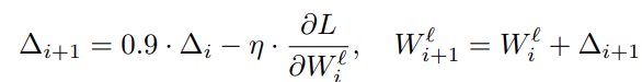
In the above formula, \(l\) refers to the layers of the SRCNN model, \(i\) refers to the layer indices, \(\eta\) is the learning rate, and \(\frac{\delta L}{\delta W_i^l}\) is the derivative.
The Training Data Sub-Images
During training, the authors create sub-images for the T91 dataset which contains 91 images originally. Creating sub-images or patches of 32×32 with a stride of 14 results in 24,800 patches for the T91 dataset. Similarly, they do so for 395,909 images from the ILSVRC 2013 ImageNet detection training data which gives them more than 5 million training patches. We will discuss more on these lines in the experiments section.
Experiments and Results
Let’s discuss the experiments and results now. Originally, the authors experiment with two different datasets. The T91 dataset and a subset of images from the ImageNet detection training set. They use the Set5 and Set14 datasets for validation/testing. And all the PSNR plots show the test PSNR on the Set5 and Set14 datasets only, not the training PSNR.
They use the base architecture among many others others. That is, the SRCNN architecture with f1 = 9, f2 = 1, f3 = 5, n1 = 64, and n2 = 32. This architecture only has 8,032 parameters.
In all experiments, they train for the same 8×10\(^8\) backpropagations with a batch size of 128. These are the high-level results with the above network configuration:
- 32.39 dB when training on the T91 dataset.
- 32.52 dB when training on the ImageNet dataset.
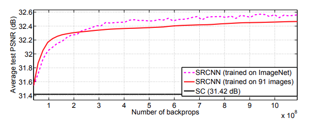
Figure 5 shows the test PSNR when training on both. the T91 and the ImageNet dataset. It is quite clear that the basic SRCNN model is easily able to beat the Sparse-Coding method.
And the following figure shows the Set5 test result comparison for SRCNN with other methods just after a few iterations of training.
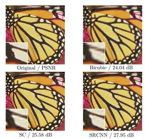
Even though the SRCNN method is not exactly as clear as the original one, it is much better compared to bicubic and Sparse-Coding methods.
Experiments with Filter Numbers
The authors also experiment with different filter numbers for \(n_1\) and \(n_2\). The following table shows the results with different filter numbers while training on the ImageNet images.
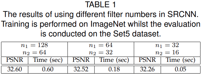
With 128 and 64 filters in the respective layers, the model is able to achieve a PSNR of 32.60 dB. This is higher compared to the other filter settings. But this also comes at the cost of running time during inference. Obviously, if a faster running time is desirable, then smaller filters will help in achieving that, but again at the cost of the quality of the super-resolved image.
Experiments with Filter Sizes
The authors carry out further experiments with filter sizes for different values of \(f1-f2-f3\). They change the filter size for \(f2\) while keeping \(f1=9\) and \(f2=5\).
With \(f2=3\), that is, with 9-3-5 setting, the test PSNR is 32.66 dB and with \(f2=5\), 9-5-5 setting, the PSNR is 32.75 dB. While the PSNR improves, the run time again increases. So, it is necessary to make a choice for the trade-off between run time and super-resolution quality.
Experiments with More Number of Layers
Further experiments include adding one more layer in-between. The following figure sums up these results.
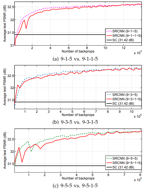
As the authors also put it, “the deeper, the better” does not hold true for the SRCNN model. Although all the four-layered networks are reaching the same PSNR, and may even surpass that given more backpropagations, the training time and increase in complexity of the network, may not make it worth it.
SRCNN Super Resolution Results Compared with Other Methods
By now, we have a good idea that SRCNN works really well, even if the network is not that deep and very simple. We have seen how it beats the Sparse-Coding methods easily.
Let’s take a look at a final graph comparing the SRCNN results with all other methods for image super resolution.
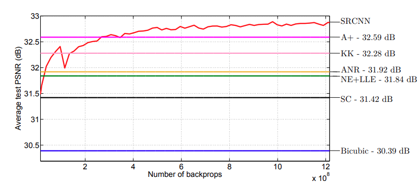
The above graph shows the test convergence of SRCNN and other methods on the Set5 dataset. We can see that the SRCNN architecture is beating all other super resolution methods by a good margin.
And finally, the running time on the Set14 dataset.
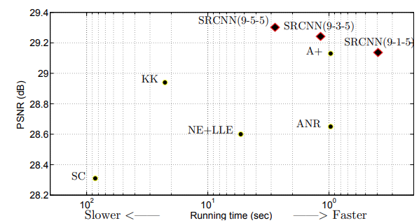
The above run time results are from a machine with an Intel CPU @ 3.10 GHz and 16 GB memory. The SRCNN(9-1-5) is the fastest among all while giving state-of-the-art PSNR. Even the SRCNN(9-5-5) and SRCNN(9-3-5) with larger filter sizes are quite fast while providing the highest test PSNR.
The above results really show the capability of the SRCNN model. It is quite amazing how such a simple and small model is able to achieve great results. This particular paper is from 2015. As of now, there are a lot of improved methods of super resolution including GANs (SRGAN is one of them). Hopefully, we will be able to cover a lot of them in future posts and also check out the code implementation for them.
Summary and Conclusion
In this post, we discussed the Image Super Resolution Using Deep Convolutional Networks paper. We started with the very basic definition of image super resolution and ended with the experiment results from the paper. In future tutorials, we will implement the SRCNN architecture and a few experiments with the PyTorch deep learning framework. I hope that this post was helpful to you.
If you have any doubts, thoughts, or suggestions, please leave them in the comment section. I will surely address them.
You can contact me using the Contact section. You can also find me on LinkedIn, and X.

great job
Thank you.