
Many of you must have used ResNets for image classification numerous times. And if you are in the field of deep learning for quite some time now, then chances are that you have ResNets as a backbone for object detection as well. But many newcomers in the field of deep learning find it difficult to grasp the concept of Residual Neural Networks or ResNets for short. They even use it for many image classification projects but find it hard to know why they work so well. In this article, we will go through the important bits of Residual Neural Networks (ResNets) in deep learning. We will do so by the best means possible, that is going through the paper in detail.
The original ResNet paper is called Deep Residual Learning for Image Recognition.
In this article, we will try to answer three important questions.
- What are ResNets in deep learning?
- What problems do ResNets solve in deep learning?
- Why do they work so well?
So, let us jump into the article now.
ResNets in Deep Learning
We will be going through the paper Deep Residual Learning for Image Recognition by Kaiming He et al. in this article. Deep Residual Neural Networks or also popularly known as ResNets solved some of the pressing problems of training deep neural networks at the time of publication.
In simple words, they made the learning and training of deeper neural networks easier and more effective. Along with that, ResNets also became a baseline for image classification benchmarks.
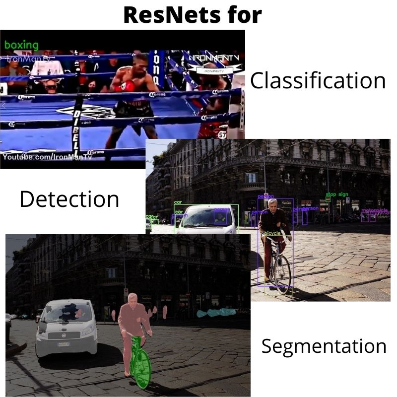
Not only that, deep learning researchers and practitioners started to use pre-trained ResNets and get really good results by fine-tuning on many deep learning projects and datasets. They even proved to be a great backbone for object detection models. And they beat some of the best state-of-the-art models like VGG nets. Along with that, the results from ResNets also won 1st place on the ILSVRC 2015 classification task.
So, what is it that made ResNets so much better than the previous deep learning models? Was it more layers? Was it more training parameters? We will try to answer these questions further on in this article.
Problems with Deeper Networks in Deep Learning
When deep learning started to become popular, then building deeper neural networks with more layers was thought to be the solution to more complex problems and datasets.
But soon (somewhere around 2015), it became clear that building deeper neural networks with more layers is not the perfect solution for every new problem.
The following are some of the problems that deep learning researchers started to face when training really deep neural networks with hundreds of millions of parameters.
- With the increase in layer depth, the neural network model does not necessarily perform better. After a certain point, the complexity started to increase and accuracy started to decrease.
- More layers mean more parameters, which means longer training time. This needs more computational power as well.
- When deeper networks start to converge, then the accuracy starts to saturate and then start to degrade after some time as well.
- There is also the problem of vanishing gradients with deeper networks.
- Higher training error after reaching certain accuracy and overfitting also seen in deeper neural networks.
- Very deep neural networks are also hard to optimize.
These are a lot of problems. And concepts like Batch Normalization also solved some of the issues like the vanishing gradients problem. Dropout also helped to reduce the overfitting of very deep neural networks.
But some of the pressing problems like degradation in accuracy, increase in training error, and harder optimization issues were still there.
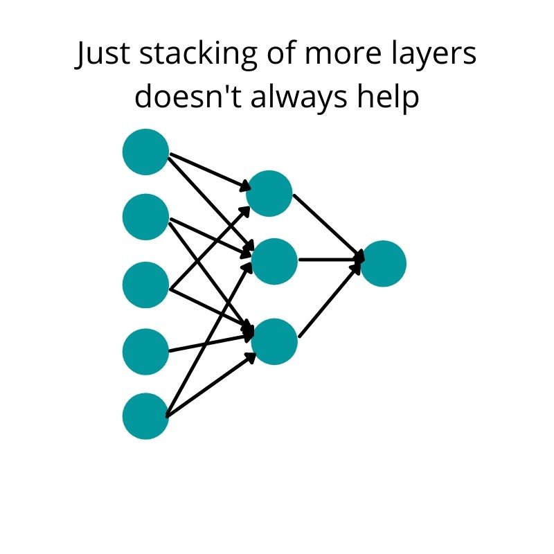
By now it was pretty clear that only stacking of more layers is not the solution to more complex problems and datasets in deep learning. And the Residual Neural Networks really come to the rescue here. So, the authors of the paper address the issue of degradation of learning capability by using a deep residual learning framework.
How Residual Neural Networks (ResNets) Help Solve the Issues?
While learning about ResNets, we will focus on two terms mainly.
- Skip connections or shortcut connections.
- Identity mapping.
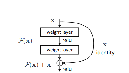
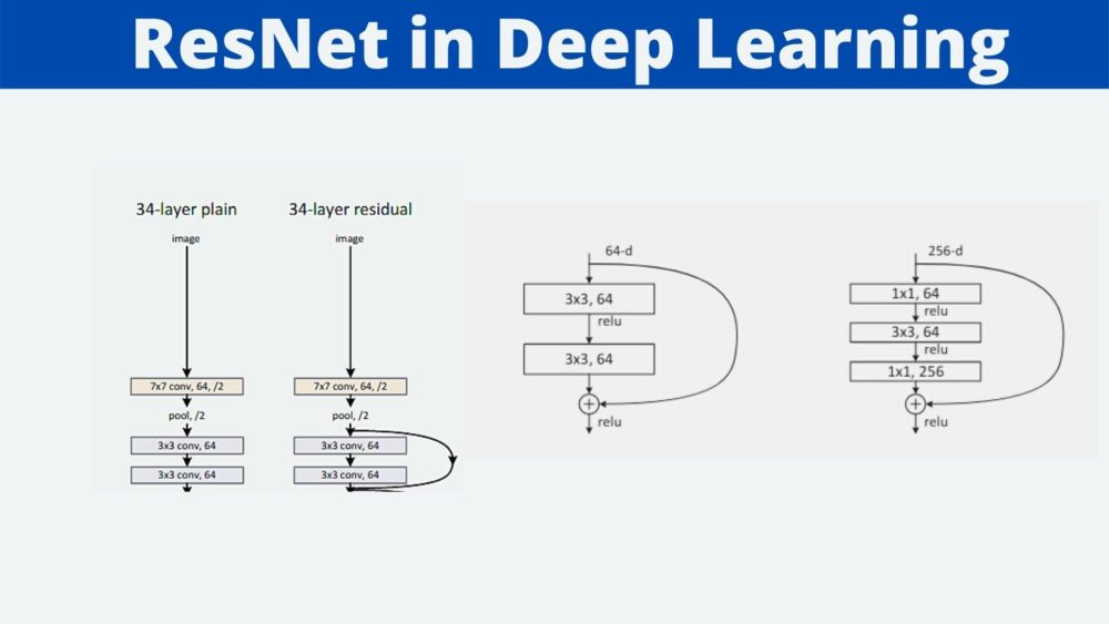
Basically, ResNets apply identity mapping between layers to achieve the shortcut connections architecture. And the layers/block in the architecture which consist of these shortcut connections are known as residual learning blocks (figure 4).
So, what does the above sentence actually mean and how do we formulate it? Let us see that in the next sub-section.
Deep Residual Learning with Skip Connections
Let us consider that \(x\) is the input to our neural network. After passing through some layers, we have the intermediate mapping to be \(\mathcal{H}(x)\). And we get this by passing the input \(x\) through some function \(\mathcal{F}\).
$$
\mathcal{F}(x) = \mathcal{H}(x)
$$
And if we consider \(y\) to be output, then we can say the following as well.
$$
y = \mathcal{F}(x)
$$
The above equations show how normal neural networks map the input to the intermediate representation and then to the output \(y\).
But how does this process change in the learning of Residual Neural Networks (ResNets)? If you take a look at figure 4 again, then you will notice that the so called residual block is consisting of two layers. And the input to the second layer is output from the first as well as the input from the first layer. That extra input is actually called the identity mapping which we have been discussing about.
According to the above structure, our former equation changes to the following.

\(y = \mathcal{F}(x) + x\)
Although, there are a few more details to know about here. We know that in simple neural networks, the function \(\mathcal{F}\) generally means multiplying some weights \(W\) with the input \(x\). This means that \(y = Wx\). And if we change that to a residual learning block with skip connections, then we get the following.
$$
y = Wx + x
$$
But in the above block, we see that we have two layers and even a ReLU non-linearity. And notice that the ReLU is applied before the second layer and again after the identity mapping. This means, that we have two sets of weight vectors, \(W_1\) and \(W_2\) for the two layers. And along with the residual learning and skip connection, our new equation will look like the following.
$$
y = W_2\sigma(W_1x) + x
$$
In the above equation, \(\sigma\) denotes the ReLU non-linearity.
So, the operation, \(\mathcal{F} + x\) is performed by the shortcut connection and then the element-wise addition operation is done. And if you look at the above figures, then you will know that we are also applying a second non-linearity to the entire block, making the final result as \(\sigma(y)\).
What if the Input and Output in a Residual Block are of Different Dimensions?
Now, we also know that convolution operations tend to reduce the dimensions of feature maps. But for the identity mapping, the dimension of \(x\) and \(\mathcal{F}\) must be equal.
In such cases, we have to perform some operation on \(x\) before doing the identity mapping which will make it the same dimension as that of \(\mathcal{F}\). For that, we can perform a linear projection using a set of weights \(W_s\) through the shortcut connection. To create a linear projection, we can use 1×1 convolution operation. The following image will give us some clear insights.
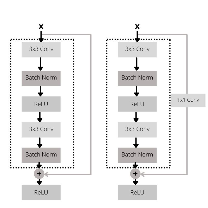
And the equation will change to the following.
$$
y = \mathcal{F}x + W_sx
$$
The above sums the concept of residual learning and shortcut connections in ResNets. I hope that everything is clear up to this point.
By now, we know how residual blocks are stacked in ResNets. But how do they help with the reduction of the issues that we discussed above?
How Do Residual Neural Networks Help?
The very basic thinking behind working of ResNets is that they help solve the problem of vanishing gradients. But if we think about it, then the vanishing gradient problem had largely been solved using batch normalization even before ResNets existed. Even the authors from the ResNet paper confirm that.
We argue that this optimization difficulty is unlikely to be caused by vanishing gradients. These plain networks are trained with BN [16], which ensures forward propagated signals to have non-zero variances. We also verify that the backward propagated gradients exhibit healthy norms with BN. So neither forward nor backward signals vanish.
Deep Residual Learning for Image Recognition, Kaiming He et al.
This means that Residual Neural Networks do not exactly solve the problem of vanishing gradients. So, how do they help?
First of all, they help reduce the training error faster and the convergence rates are higher even if the layer depths keep on increasing in the neural networks. Secondly, this in turn helps in easier optimization. But according to the paper and authors, this is also just speculation. Most probably, identity mapping helps in some ways which still needs to be studied carefully.
Different Residual Neural Network Architectures
In this section, we will discuss the different ResNet architectures and how the shortcut connections are used in the networks.
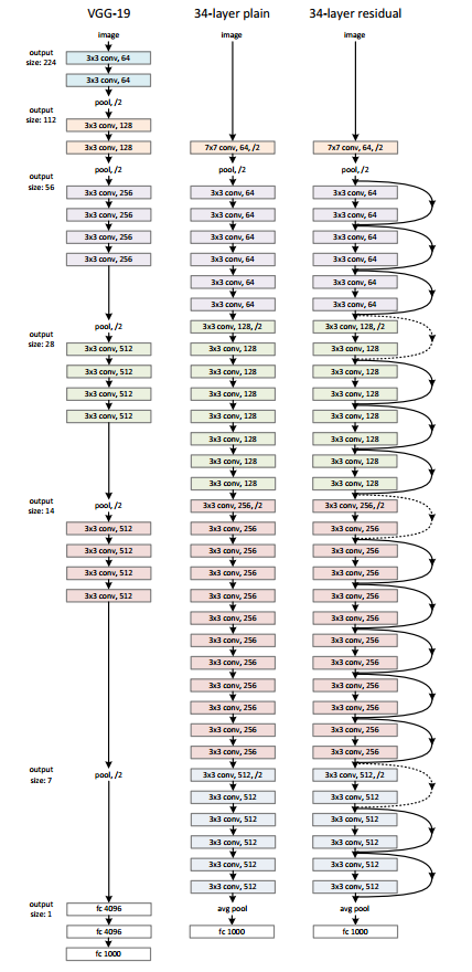
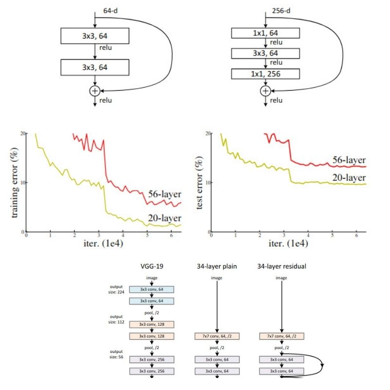
Figure 6 shows a 34 layered Residual Neural Network (on the right) also commonly known as ResNet-34. It is shown alongside the famous VGG 19 and a plain 34 layer deep neural network.
In the ResNet-34 network, we can see the shortcut connections between the layers very clearly. If you observe carefully, you will see two different lines, one solid and one dotted for the shortcut connections. The dotted lines indicate an increase in the dimensions. You might ask “why compare the three models side by side?”
Note that VGG 19 has 19 layers in total with 19.6 billion FLOPs which is a big number. The plain neural network with 34 layers has only 3.6 billion FLOPs. And the ResNet-34 with the shortcut connections also has 3.6 billion FLOPs. You see, the shortcut connections do not add to the computation of a neural network and they have all the added advantages for sure.
Along with the 34 layered ResNet, we also have ResNet variants for 18, 50, 101, and 152 layers respectively. You make take a look at the following figure to get a good idea.
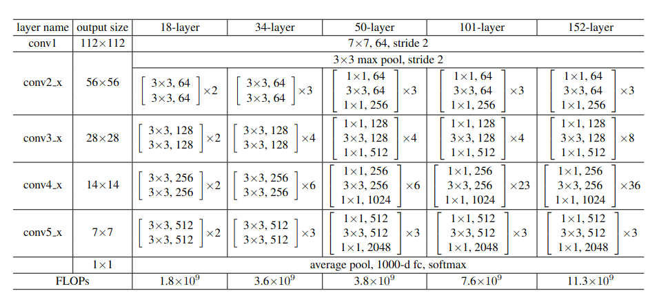
There is a very interesting thing to notice in figure 7. Even one of the largest Residual Neural Network architecture, that is, ResNet-101, has less number of FLOPs (11.3 billion) when compared to VGG 19. This fact will become even more interesting when we see the results of Residual Neural Networks in the next section.
Experiments and Results from the Paper
The authors have performed a number of experiments, both on the ImageNet dataset and the CIFAR-10 dataset. Let us take a look at a few of them.
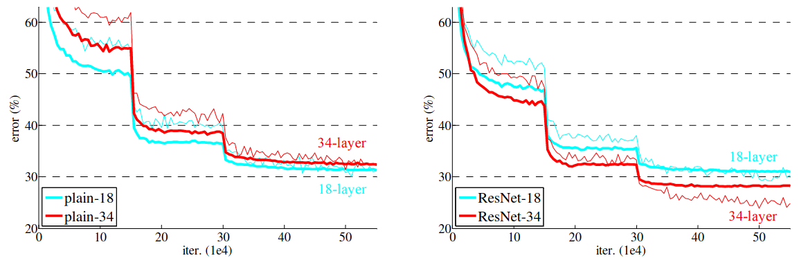
Figure 8 shows the training comparison of the plain 18 layer & 34 layer neural networks with that of ResNet-18 and ResNet-34. The bold curves show the validation error. And we can see that in the case of plain networks the 18 layered network has less error than that of the 34 layered network. This indicates the degradation in performance that deeper neural networks suffer from. Whereas in the case of ResNets, ResNet-34 has a lower validation error.
| plain | ResNet | |
| 18 layers | 27.94 | 27.88 |
| 34 layers | 28.54 | 25.03 |
Table 1 also shows the outputs that support the facts from figure 8 with the training errors for the plain networks and the ResNets. ResNet-34 has the lowest error as discussed above.
Now, let us take a look the validation error rates and their comparison of different models for the ImageNet validation set.
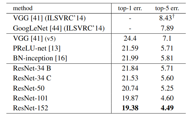
Figure 9 shows the validation error rates for various single models on the ImageNet dataset. We can see that VGG has a top-5% error rate of 8.43. And this most probably is the result for VGG 19. And there is also the improved VGG (v5) with error rate of 7.1 But with that also, all the ResNet models have lower top-5% error rates, even the ResNet-34 networks. This is quite amazing.
It is very clear that Residual Neural Networks proved to be superior to the previous models which just stacked layers one after the other. The identity mapping and shortcut connections surely help.
There are many other results discussed in the paper as well, along with object detection experiments on the MS COCO dataset. If you are interested, then please take a look at the paper.
Advantages of Residual Neural Networks
We have covered a lot about ResNets till now. Starting from the identity mapping, the shortcut connections, the architectures, some experimental results as well.
For the final part, let us point out what benefits and advantages that ResNets offer.
- With ResNets, learning continues even as the depth of networks grows. ResNet-101 and ResNet-152 are very concrete proofs of it.
- Deeper residual networks provide better learning capability and better convergence also.
- No increase in the number of parameters when compared to non-ResNet architectures with same number of layers. That is, identity mapping does not introduce any additional computation complexity.
- Less training error when compared to counterpart plain nets.
- Residual Neural Networks are easy to optimize and work very well with standard optimizers like SGD (Stochastic Gradient Descent).
The above are some very good pointers that should encourage deep learning practitioners to leverage the power of ResNets.
If You Want to get Hands-On with ResNets…
If you really want to get your hands dirty with code and train ResNets using PyTorch, you can refer to some of the following posts.
- Action Recognition in Videos using Deep Learning and PyTorch.
- Advanced Facial Keypoint Detection with PyTorch.
- Many more… click here.
Summary and Conclusion
In this blog post, we learned about Deep Residual Neural Networks by going through the original paper and the results. We saw how ResNets help in deep learning training and what are the different architectures of ResNets. We also learned about shortcut connections and identity mapping in ResNets. I hope that you learned something new from this article.
If you have any doubts, thoughts, or suggestions, then please leave them in the comment section. I will surely address them.
You can contact me using the Contact section. You can also find me on LinkedIn, and X.

6 thoughts on “Residual Neural Networks – ResNets: Paper Explanation”