Implementing VGG11 from Scratch using PyTorch

In deep learning, we use pre-trained models all the time for fine-tuning and transfer learning on newer datasets. If not pre-trained models, then most of the time we use pre-defined models from well-known libraries like PyTorch and TensorFlow and train from scratch. But it is also important to know how to implement deep learning models from scratch. If not all, at least some of the well-known models. That is why we will be implementing the VGG11 deep learning model from scratch using PyTorch in this tutorial.

We will implement the VGG11 deep neural network as described in the original paper, Very Deep Convolutional Networks for Large-Scale Image Recognition by Karen Simonyan and Andrew Zisserman. This paper introduced the VGG models in deep learning. I highly recommend that you go through the paper at least once on your own also.

This post is going to be a three part series.

• This week (part one): Implementing VGG11 from scratch using PyTorch.
• Next week (part two): Training our implemented VGG11 model from scratch.
• Final part (part three): Implementing all the VGG models in a generalized manner using the PyTorch deep learning framework.

So, what are we going to learn in this tutorial?

• The VGG11 Deep Neural Network Model.
  • Knowing about the model architectures.
  • Knowing about the different convolutional and fully connected layers.
  • The number of parameters.
  • Implementation details.
• Implementing VGG11 from scratch using PyTorch.

I hope that you are excited to follow along with me in this tutorial.

The VGG11 Deep Neural Network Model

In the paper, the authors introduced not one but six different network configurations for the VGG neural network models. Each of them has a different neural network architecture. Some of them differ in the number of layers and some in the configuration of the layers.

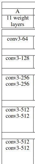
In this blog post, we are going to focus on the VGG11 deep learning model. It is the simplest of all the configurations. It has 11 weight layers in total, so the name VGG11. 8 of them are convolutional layers, and 3 are fully connected layers.

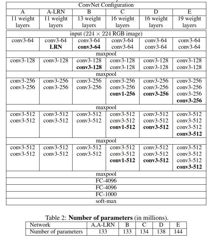
Figure 2 shows all the network configurations of the VGG neural networks. Our focus will be on the VGG11 model (configuration A). The main reason being, it is the easiest to implement and will form the basis for other configurations and training for other VGG models as well.

We can also see that VGG11 has 133 million parameters. Actually, the number is 132,863,336 to be exact. We will compare the number of parameters of our implemented model with this number to ensure that our implementation is correct.

Implementation Details

We are going to closely follow the original implementation for the VGG11 in this tutorial. This means that we will not be applying batch normalization as is suggested to do in the recent implementations of VGG models. Truly speaking, there is no reason not to include batch normalization. It’s just that “let’s implement a deep learning model from scratch as given in the paper”.

It was not included in the paper, as batch normalization was not introduced when VGG models came out. So, all the newer VGG implementations are having batch normalization as they prevent the vanishing gradient problem. But we will follow the paper to the word (just for learning).

All the other implementation details are also going to match the paper. This includes the convolutional layers, the max-pooling layers, the activation functions (ReLU), and the fully connected layers. Else, it won’t be called an implementation of VGG11.

So, our implementation of VGG11 will have:

• 11 weight layers (convolutional + fully connected).
  • The convolutional layers will have a 3×3 kernel size with a stride of 1 and padding of 1.
• 2D max pooling in between the weight layers as explained in the paper. Not all the convolutional layers are followed by max-pooling layers.
• ReLU non-linearity as activation functions.

Implementing VGG11 from Scratch using PyTorch

From this section onward, we will start the coding part of this tutorial.

Before moving forward, let’s take a closer look at the VGG11 architecture and layers.

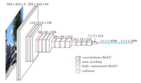
Above, Figure 3 shows the VGG11 model’s convolutional layers from the original paper. Note that the ReLU activations are not shown here for brevity.

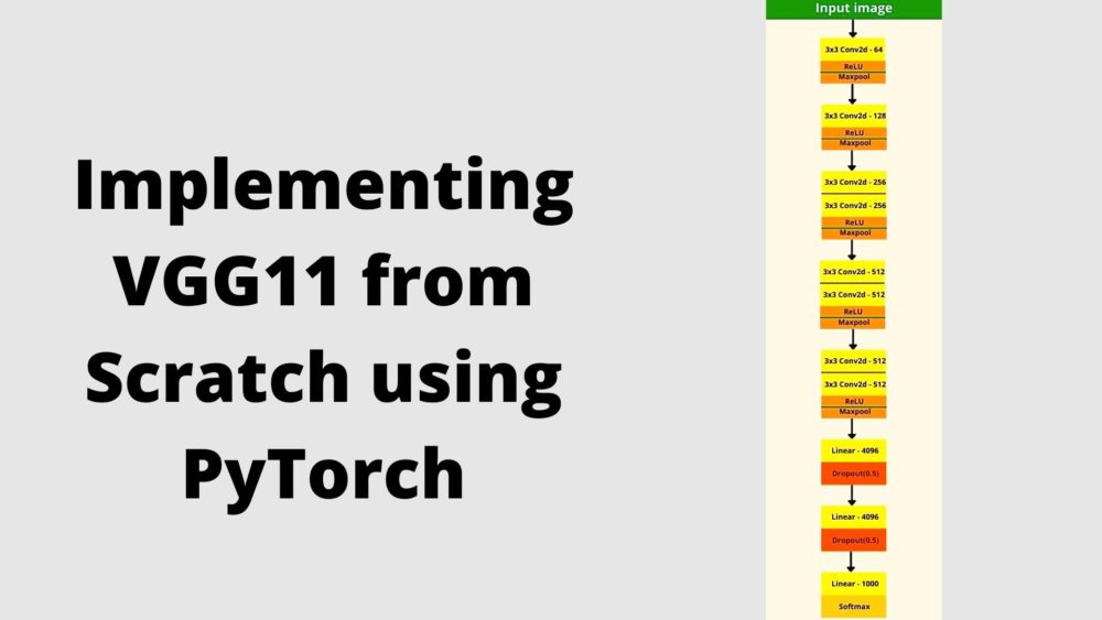
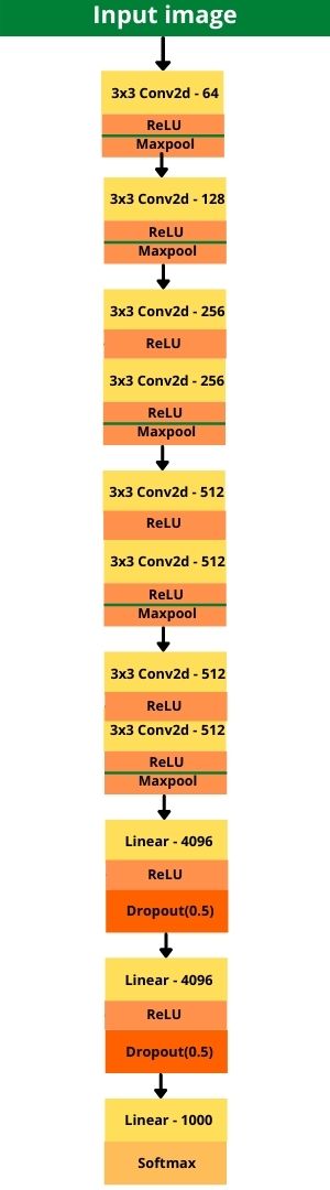
Figure 4 shows the complete block diagram of VGG11 which includes all the layers as we are going to implement them.

I hope that figure 4 gives some more clarity and helps in the visualization of how we are going to implement it. Please note that figure 4 contains Dropout layers after the fully connected linear layers which are not shown in the original table given in the paper. But dropout has been used in the original implementation as well.

Coding VGG11 with PyTorch

Let us start coding VGG11 with PyTorch.

We just need one Python script file for this tutorial. You can create a Python file in any project folder that you want and give an appropriate name. I have named the Python file as vgg11.py.

Importing the Required Modules

We do not require a lot of libraries and modules for the VGG11 implementation. In fact, we need only two PyTorch modules in total.

import torch
import torch.nn as nn

We only need the torch module and the torch.nn module.

The VGG11 Model Class

Next, we will implement the VGG11 model class architecture. We will call it VGG11(). The next block of code is going to be a bit big as it contains the complete VGG11 class code. This will ensure continuity and indentation of the code, and will also avoid a lot of confusion. We will get into the explanation of the code after writing it.

# the VGG11 architecture
class VGG11(nn.Module):
    def __init__(self, in_channels, num_classes=1000):
        super(VGG11, self).__init__()
        self.in_channels = in_channels
        self.num_classes = num_classes

        # convolutional layers 
        self.conv_layers = nn.Sequential(
            nn.Conv2d(self.in_channels, 64, kernel_size=3, padding=1),
            nn.ReLU(),
            nn.MaxPool2d(kernel_size=2, stride=2),
            nn.Conv2d(64, 128, kernel_size=3, padding=1),
            nn.ReLU(),
            nn.MaxPool2d(kernel_size=2, stride=2),
            nn.Conv2d(128, 256, kernel_size=3, padding=1),
            nn.ReLU(),
            nn.Conv2d(256, 256, kernel_size=3, padding=1),
            nn.ReLU(),
            nn.MaxPool2d(kernel_size=2, stride=2),
            nn.Conv2d(256, 512, kernel_size=3, padding=1),
            nn.ReLU(),
            nn.Conv2d(512, 512, kernel_size=3, padding=1),
            nn.ReLU(),
            nn.MaxPool2d(kernel_size=2, stride=2),
            nn.Conv2d(512, 512, kernel_size=3, padding=1),
            nn.ReLU(),
            nn.Conv2d(512, 512, kernel_size=3, padding=1),
            nn.ReLU(),
            nn.MaxPool2d(kernel_size=2, stride=2)
        )

        # fully connected linear layers
        self.linear_layers = nn.Sequential(
            nn.Linear(in_features=512*7*7, out_features=4096),
            nn.ReLU(),
            nn.Dropout2d(0.5),
            nn.Linear(in_features=4096, out_features=4096),
            nn.ReLU(),
            nn.Dropout2d(0.5),
            nn.Linear(in_features=4096, out_features=self.num_classes)
        )

    def forward(self, x):
        x = self.conv_layers(x)
        # flatten to prepare for the fully connected layers
        x = x.view(x.size(0), -1)
        x = self.linear_layers(x)
        return x

As you can see, our VGG11 class contains the usual methods present in a PyTorch neural network class code. They are the __init__() method and the forward() method. Let us go over the code in detail.

The __init__() Method

• It is accepting the in_channels and num_classes parameters which are the number of color channels for the image and the number of output classes for the dataset. We will have to pass the number of channels while initializing the VGG11 model depending upon the type of images that we are using. It is going to be 3 for RGB images and 1 for grayscale images. And as the original VGG models were benchmarked on the ImageNet dataset with 1000 classes, therefore, our initial value is 1000 as well. We can change this value while initializing the model.
• Starting from line 11 we have all the convolutional layer definitions. We have used the Sequential class from the torch.nn module so that we can stack the layers properly along with the ReLU and max-pooling layers. This makes the code much cleaner.
• The first Conv2d() layer has in_channels as self.in_channels that we have initialized above. The out_channels is 64 as per the paper. The kernel size is 3 and padding is 1 which is also according to the paper.
• This is followed by the ReLU activation function and the 2D max-pooling. The max-pooling layers have a kernel size of 2 and a stride of 2.
• After that, we keep on increasing the output channel size till we reach a value of 512 for the final convolutional layer.
• There is one thing to note here. Each convolutional layer is followed by a ReLU activation but the max-pooling layers are not defined after each convolution. Please do take note of the places where the max-pooling layers are defined.
• The final convolutional layer has 512 output channels and is followed by the ReLU activation and max-pooling as usual.

Also, we need to keep in mind that the max-pooling layers to going to halve the feature maps each time. And we have 5 such max-pooling layers with a stride of 2. This is going to be important when we will be implementing the fully connected layers.

Coming to the fully connected layers. We have defined a self.linear_layers and used the Sequential block to define all the fully connected linear layers.

• The fully connected blocks are the same for all the VGG architectures. They contain three fully connected layers.
• The first linear layer has 512*7*7 input features. But how did we reach here? Note that VGG takes an input size of 224×224 (height x width) for images. And we have 5 max-pool layers with a stride of 2 which are going to halve the features maps each time. Also, the final convolutional layer has 512 output channels. To get the number of input features for the first Linear() layer, we just need to calculate it using the following formula.
  • 224 / (2^5) = 7
  • And because the final convolutional layer has 512 output channels, the first linear layer has 512*7*7 input features.
• After the ReLU activation, we are also using Dropout with a probability of 0.5. You will not find the mention of dropout in the architecture table in the paper. Instead, it is mentioned in Section 3 in the paper under the Training sub-heading. And therefore, we are also using it in our implementation.
• After that, we have another Linear() layer with 4096 output features. And the final Linear() layer has the number of classes as output features. Initially, it is 1000. We can change it according to our dataset when initializing the model.

The forward() Method

The forward() method is pretty simple to follow along.

• At line 47, we forward propagate the image tensor through all the convolutional layers (self.conv_layers). This provides us with all the feature maps.
• Then at line 49, we flatten the feature maps and pass them through the linear layers (self.linear_layers).
• Finally, we return the softmax outputs.

This completes our VGG11 deep neural network model.

Checking Our VGG11 Implementation for Correctness

Our implementation of the VGG11 model is complete. The final thing that is left is checking whether our implementation of the model is correct or not.

We can do that very easily.

• First, we will calculate the number of parameters of our model. It should be equal to 132,863,336.
• Second, we will forward propagate a dummy tensor input through our model and check the output size. It should be equal to (1, 1000), indicating that we have outputs for 1000 classes.

Let us write the code for that.

if __name__ == '__main__':
    # initialize the VGG model for RGB images with 3 channels
    vgg11 = VGG11(in_channels=3)
    # total parameters in the model
    total_params = sum(p.numel() for p in vgg11.parameters())
    print(f"[INFO]: {total_params:,} total parameters.")
    
    # forward pass check
    # a dummy (random) input tensor to feed into the VGG11 model
    image_tensor = torch.randn(1, 3, 224, 224) # a single image batch
    outputs = vgg11(image_tensor)
    print(outputs.shape)

The above code will be executed only if we execute the vgg11.py Python script directly. Importing the script as a module will not run the above code block.

• At line 54, we are initializing the VGG11 model. Then we are computing the total number of parameters and printing the value as well.
• Starting from line 61, we define a dummy input tensor called image_tensor. Then we are forward propagating this through the model and printing the shape of the outputs.

Now we can execute the vgg11.py script and check the outputs that we are getting. Open the terminal/command prompt in the current working directory and execute the following command.

python vgg11.py 

You should see the following output.

[INFO]: 132,863,336 total parameters.
torch.Size([1, 1000])

We are getting the total number of parameters as 132,863,336 and the output size as (1, 1000). This ensures that our implementation of VGG11 deep neural network model is completely correct.

If you wish you can also run the above tests on your CUDA enabled GPU. You just need to change a couple of lines.

if __name__ == '__main__':
    # initialize the VGG model for RGB images with 3 channels
    vgg11 = VGG11(in_channels=3).cuda()
    # total parameters in the model
    total_params = sum(p.numel() for p in vgg11.parameters())
    print(f"[INFO]: {total_params:,} total parameters.")
    
    # forward pass check
    # a dummy (random) input tensor to feed into the VGG11 model
    image_tensor = torch.randn(1, 3, 224, 224).cuda() # a single image batch
    outputs = vgg11(image_tensor)
    print(outputs.shape)

We are just loading the model and the dummy tensor on to the CUDA device. You can execute the script again using the same command and it should run fine while giving the correct outputs.

Summary and Conclusion

In this blog post, we went through a short tutorial of implementing VGG11 model from scratch using the PyTorch deep learning framework. In the next blog posts, we will see how to train the VGG11 network from scratch and how to implement all the VGG architectures in a generalized manner. I hope that you learned something new from this tutorial.

If you have any doubts, thoughts, or suggestions, then please leave them in the comment section. I will surely address them.

You can contact me using the Contact section. You can also find me on LinkedIn, and Twitter.