Image Classification using TensorFlow Pretrained Models

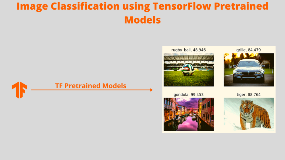
In this tutorial, you will be learning how to carry out image classification using pretrained models in TensorFlow.

This is the seventh post in the series, Getting Started with TensorFlow.

• Introduction to Tensors in TensorFlow.
• Basics of TensorFlow GradientTape.
• Linear Regression using TensorFlow GradientTape.
• Training Your First Neural Network in TensorFlow.
• Convolutional Neural Network in TensorFlow.
• Image Classification using TensorFlow on Custom Dataset.
• Image Classification using TensorFlow Pretrained Models.

If you are new to TensorFlow, going through the previous posts will surely help you. In fact, starting from the first post is an even better idea. I am sure that you will be able to learn a lot. You will learn about tensors in TensorFlow, how to represent tensors with different ranks, and even carrying out tensor operations on the GPU.

In this post, we will cover the following topics.

• We will start with a brief introduction to the models that we will use for image classification.
  • ResNet.
  • VGG.
  • MobileNet.
• Then we will start the coding part of the tutorial where we will use all three of these models for image classification.
• Finally, we will end with what we learn in this post and how to take this learning one step further.

I hope that you are excited to follow along with the tutorial. Let’s jump into it then, without any more delay.

First, we will discuss ResNets, VGG nets, and MobileNet architectures in short. Then we will move over to the coding part of the tutorial.

VGG

The VGG models were introduced in the paper Very Deep Convolutional Networks for Large-Scale Image Recognition by Karen Simonyan and Andrew Zisserman.

At the time, the VGG models were state-of-the-art for image classification tasks. The models performed really well in the ImageNet 2014 challenge securing first and second places in localization and classification tasks respectively.

This shows that VGG models were not only suitable for image classification but also for object detection.

In the paper, the authors introduced not one but 6 different models.

We can see there are 6 models, starting from VGG11 to VGG19. The number in the name indicates the number of weight layers present in that particular model.

As we can see, all the model architectures are pretty simple. The models are simple stacking of 3×3 convolutional layers, max-pooling layers, and fully connected layers, followed by a final softmax output.

The only difference in all the models is only in the convolutional layers. All the models have three fully connected layers with the final one having 1000 units. This 1000 corresponds to the 1000 classes in the ImageNet classification dataset. Needless to say, we can easily modify the final fully connected layer according to our own requirements also.

Please consider the following tutorials if you want to learn the practical implementation of VGG models using PyTorch.

Implementing VGG11 from Scratch using PyTorch

Training VGG11 from Scratch using PyTorch

Implementing VGG Neural Networks in a Generalized Manner using PyTorch

ResNet

Residual Neural Networks or ResNets first came into the picture through the paper Deep Residual Learning for Image Recognition by Kaiming He et al.

ResNets helped to mitigate some of the pressing problems when training deep neural networks. Like:

• The saturation of accuracy after training for a few epochs.
• Problem of vainshing gradients.
• Increase in training error after training for certain epochs and reaching a certain accuracy.

Along with the above, the Residual Neural Networks also helped solved a few other problems as well.

But how did the authors achieve this? Instead of just stacking one neural network layer after the other, they chose a different path. The authors used:

• Skip connections.
• Identity mapping.

The authors used skip connections and identity mapping to come up with a residual learning block.

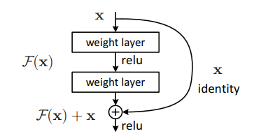
Residual Neural Networks apply identity mapping between layers to achieve short connections. The blocks which consist of these connections are known as the residual learning blocks.

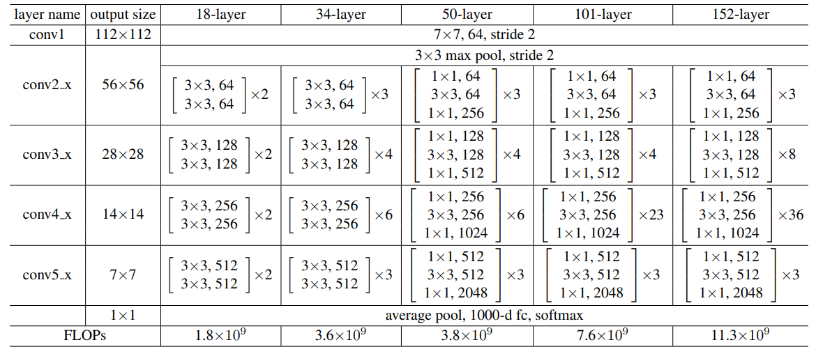
In fact, the authors came up with five different ResNet architectures namely:

• ResNet18.
• ResNet34.
• ResNet50.
• ResNet101.
• ResNet152.

Also, the ResNet architectures were able to beat the previous simple neural networks like VGG networks in terms of accuracy when trained on the ImageNet dataset.

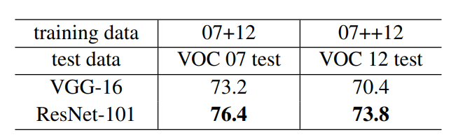
Along with classification tasks, the Residual Neural Network models also have good generalization performance on object detection tasks. They are a very good choice of backbone for state-of-the-art object detection models like Faster RCNN.

If you want to learn about ResNet in detail and know more about the paper, then consider going through the following post.

Residual Neural Networks – ResNets: Paper Explanation

MobileNets

Neural networks models like VGG nets and ResNets are quite large and deep. They run quite well on devices having good compute resources. And GPUs are quite capable of that.

But we also need models which are less compute-intensive and run on mobile and embedded devices.

MobileNets, introduced in the paper MobileNets: Efficient Convolutional Neural Networks for Mobile Vision Applications by Howard et al. are just perfect for that.

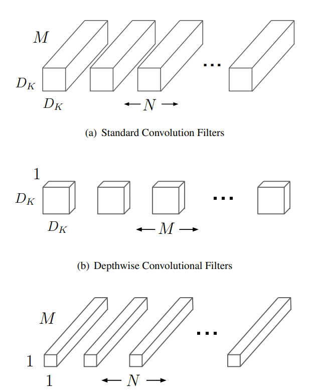
MobileNets use depthwise separable convolution that leads to lightweight yet deep neural networks.

Although many new lightweight neural networks have come up since the first publication of MobileNets. Still, we can say that they are some of the first models catering to deep learning in computer vision for mobile devices which led to further improvement.

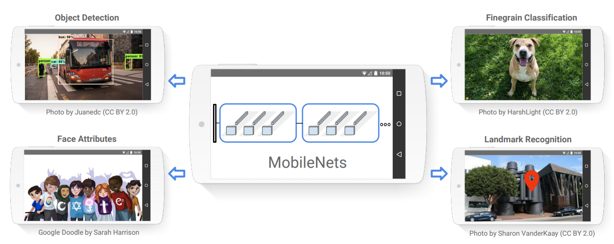
MobileNets are quite effective for a wide range of vision applications that benefit from deep learning and neural networks. The applications range from object detection to image classification, to face applications, and even large-scale geo-localization.

The two methods which make MobileNets so effective are Depthwise convolution and pointwise convolution.

We will not dive into the details of the paper or the approach here. This will require a separate post to give proper justice to the explanation. Still, the paper is quite interesting and if you want to jump into the details, you should surely give the paper a read.

TensorFlow PreTrained Models for Image Classification

Till now, we have discussed VGG nets, ResNets, and MobileNets in brief. And we know that we will be using these models for image classification.

Fortunately, TensorFlow already provides versions of these models which have been pretrained on the ImageNet dataset. This means that we can run a forward pass through any of these models by providing an image, and there is a very high chance that the model will be able to predict the class of the image from its wide range of 1000 classes.

TensorFlow has a host of other pretrained models as well. You can visit the official docs to get the entire list.

Although in this post, we will focus on VGG16, ResNet50, and MobileNetv2.

Directory Structure

We will use the following directory structure in this tutorial.

├── image_classification.py
├── input
│   ├── image_1.jpg
│   ├── image_2.jpg
│   ├── image_3.jpg
│   └── image_4.jpg
├── outputs
│   ...

• We have one Python script. This will contain the code to classify images using the three TensorFlow pretrained models.
• Then we have the input folder which contains the images we will use for classification. This contains four images on which we will run the image classification models.
• Finally, we have the outputs folder that will contain the classified image outputs after passing through the neural network models.

Now that we are done with all the preliminary stuff, let’s jump into the coding part of the tutorial.

Image Classification using TensorFlow Pretrained Models

All the code that we will write, will go into the image_classification.py Python script.

Required Imports

Let’s start by importing all the libraries and modules that we will need along the way.

import tensorflow as tf
import matplotlib.pyplot as plt
import glob as glob
import numpy as np
import argparse

• We will use matplotlib to create the final subplot of the images with the predicted labels as the titles.
• And argparse will help us create and parse command line arguments.

Create the Argument Parser

While executing the Python script, we will provide the model name that we want to use for image classification. For that, we need to construct the argument parser.

parser = argparse.ArgumentParser()
parser.add_argument('-m', '--model', default='resnet50', 
    choices=['resnet50', 'vgg16', 'mobilenet'])
args = vars(parser.parse_args())

We can provide any three of the above choices, that is:

• resnet50.
• vgg16.
• mobilenet.

And accordingly, the appropriate pretrained model will be used.

Now, let’s create a dictionary that loads the respective model according to the model names that we pass to the command line argument while executing the script.

# model dictionary to create the mapping from model name...
# ... to actual TensorFlow model instance
models_dict = {
    'resnet50': tf.keras.applications.resnet50.ResNet50(weights='imagenet'),
    'vgg16': tf.keras.applications.vgg16.VGG16(weights='imagenet'),
    'mobilenet': tf.keras.applications.mobilenet_v2.MobileNetV2(weights='imagenet'),
}

print(f"Using {args['model']} model...")
# get all the image paths
image_paths = glob.glob('input/*')
print(f"Found {len(image_paths)} images...")

In the above code block, we have a model_dict dictionary. The keys are the model names that we pass through the command line argument. And the values are the TensorFlow classes that load the corresponding image classification models. We can do so by using tf.keras.applications.

One thing to note in the above code block is the weights argument that we are passing while loading the model. This implies that we are loading the imagenet weights as the model has been pretrained on the ImageNet dataset. If we provide weights=None, then the weights will be initialized randomly and the model will not be able to classify the image correctly.

After the model_dict dictionary:

• We are printing the pretrained model that we are using for image classification on line 18.
• Using glob to store all the image paths in the image_paths list on line 20. And printing the total number images that we have.

Classify the Images using TensorFlow Pretrained Models

Next, we will read the images, and pass them through the model to get the predictions. This follows a few simple steps.

• Loop through each of the image paths.
• Load and resize the image to appropriate dimensions.
• Further preprocess the image using TensorFlow utilities.
• Load the pretrained model according to the model names passed through the command line argument.
• Forward pass the image through the pretrained model to get the intitial predictions.
• Process the predictions using TensorFlow’s ImagetNet utilities to get the final predictions.
• Create a subplot of all the images with the predicted label as the title.

The above steps will become much more clearer after we write the code for it. Let’s write the code and then get to the explanation part.

for i, image_path in enumerate(image_paths):
    print(f"Processing and classifying on {image_path.split('/')[-1]}")
    # read image using matplotlib to keep an original RGB copy
    orig_image = plt.imread(image_path)
    # read and resize the image
    image = tf.keras.preprocessing.image.load_img(image_path, 
        target_size=(224, 224))
    # add batch dimension
    image = np.expand_dims(image, axis=0)
    # preprocess the image using TensorFlow utils
    image = tf.keras.applications.imagenet_utils.preprocess_input(image)

    # load the model
    model = models_dict[args['model']]
    # forward pass through the model to get the predictions
    predictions = model.predict(image)
    processed_preds = tf.keras.applications.imagenet_utils.decode_predictions(
        preds=predictions
    )
    # print(f"Original predictions: {predictions}")
    print(f"Processed predictions: {processed_preds}")
    print('-'*50)
    
    # create subplot of all images
    plt.subplot(2, 2, i+1)
    plt.imshow(orig_image)
    plt.title(f"{processed_preds[0][0][1]}, {processed_preds[0][0][2] *100:.3f}")
    plt.axis('off')

plt.savefig(f"outputs/{args['model']}_output.png")
plt.show()
plt.close()

Code Explanation

Let’s go through the code.

• On line 29, we are reading the image using Matplotlib and keeping an original copy which we will use at the end for visualization.
• Line 31 uses TensorFlow’s load_img function to read and resize the image appropriately. Generally, pretrained models require the images to be resized to a specific shape. This mostly corresponds to the size to which the ImageNet images were resized to when the models were trained on the ImageNet dataset. All the models that we use here require images of size 224×224. There are few other models like Inception networks which need images of size 299×299.
• Then we use NumPy to add an extra batch dimension to the image. This makes the image shape as 1x224x224x3.
• On line 36, we use the imagenet_utils to preproess the image properly one final time.
• Then we load the model and carry out the prediction on line 41. This gives us an intial set of 1000 predictions. We have to filter out the predictions to get the most appropriate one.
• We then use the decode_predictions function from the imagenet_utils which returns the top 5 predictions according to the confidence score by default.
• Starting from line 50, we create a subplot of the image and add the predicted label as the title. We also save the image by appending the model name to the image file path. This will help us later distinguish which models classified which images.

That’s all we need for the coding part.

Executing the Python Script

Let’s now execute the Python script with a different model flag each time. Open your terminal in the current working directory. And let’s start with the VGG16 model.

python image_classification.py  --model vgg16

The following figure shows the predictions for each of the images.

The VGG16 model predicted the gondola and tiger with pretty high confidence. It also predicted the soccer_ball correctly but with lower confidence. But for the car, it predicted is as a grille. The most plausible reason for this can be the front metal grille that is so prominent in the car image.

Let’s check with the ResNet50 model now.

python image_classification.py  --model resnet50

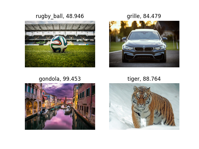
The ResNet50 model is predicting the gondola and tiger with even higher confidence. Interestingly, it is also predicting the car as grille with high confidence. But this time, it is detecting the ball as a rugby_ball instead of a soccer_ball.

Finally, the MobileNetv2 model.

python image_classification.py  --model mobilenet

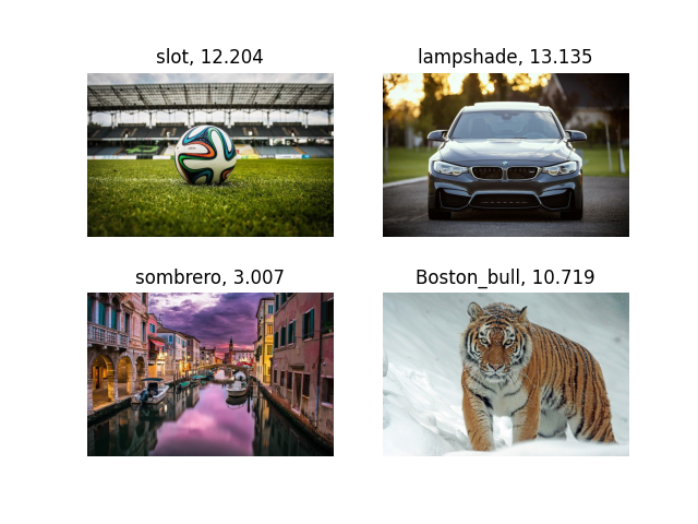
That’s odd! The MobileNetv2 model is predicting everything incorrectly. And that too with pretty much low confidence. We know that MobileNets are smaller models meant for lower accuracy and faster predictions. But not predicting even a tiger correctly is a bit strange. There are a few larger and newer versions of MobileNet like MobileNetV3 Large. Maybe you can give that model a try and see if the predictions are better.

A Few Takeaways

• We saw how different models predicted the same images with different conficdence scores. And architectures like ResNets perform better than simple VGG models.
• Also, smaller models like MobileNets may not be well suited for predicting on complex images.
• You can try a few other models like VGG19 and some Inception models as well. If you do, surely let other know in the comment section.
• You may also try larger versions of MobileNets like the MobileNetV3 Large model and check whether it is predicting any of the images correctly.
• Also, try playing around by giving a few new images as inputs to the models. Analyze how they perform and how the image complexity affects the predictions.

Summary and Conclusion

In this tutorial, you learned about image classification using TensorFlow pretrained models. We used the VGG16, ResNet50, and MobileNetV2 models which were pretrained on the ImageNet dataset. We saw how they performed on different images and how smaller models like MobileNets perform worse than other models like VGG16 and ResNet50. I hope that you learned something new from this tutorial.

If you have any doubts, thoughts, or suggestions, then please leave them in the comment section. I will surely address them.

You can contact me using the Contact section. You can also find me on LinkedIn, and Twitter.