Linear Regression using TensorFlow GradientTape

In this tutorial, you are going to learn about linear regression using TensorFlow GradientTape.

This blog post is the third in the series Getting Started with TensorFlow.

• Introduction to Tensors in TensorFlow.
• Basics of TensorFlow GradientTape.
• Linear Regression using TensorFlow GradientTape.

In the previous post, we explored TensorFlow’s GradientTape API which helps us in carrying out automatic differentiation. If you are new to TensorFlow’s GradientTape API, then going through the previous post will surely help in understanding the concepts in this post.

Also, if you are just starting with TensorFlow, then I suggest checking out the series from the beginning. This you help you to get a clear picture of the tensors in TensorFlow.

You must have carried out simple linear regression in machine learning. Maybe you used a well-known library like Scikit-Learn for that. But let’s change things a bit. We will not use Scikit-Learn in this tutorial. We will use the TensorFlow deep learning framework which is already very well known for its deep learning functionalities like image recognition, object detection, and image segmentation among many others. For carrying out simple linear regression, we will use its GradientTape API which was introduced starting from TensorFlow version 2.0 and now has become an integral part of the framework.

So, what are we going to cover in this tutorial?

• We will start off with a bit of basics of linear regression and how to map the concepts to deep learning. This includes:
  • The simple linear linear regression equation.
  • The weights and biases terms in linear regression.
• Then we will start with the coding part of the tutorial. This is where we will use TensorFlow and it’s GradientTape API to solve a simple linear regression problem on a dummy dataset.

So, let’s start with the concept of linear regression.

A Brief About Linear Regression

This section will briefly cover the basics of linear regression and try to map the concepts to machine learning. After going through this section, we will be able to easily implement linear regression using the TensorFlow GradientTape API.

In linear regression, we try to predict the values of a dependent variable using one or more independent variables. These independent variables are also called features.

When we deal with simple linear regression, then there is only one set of independent variables. This is what we will focus on in this tutorial.

Let’s start out with the equation of simple linear regression.

$$
y = mx + c
$$

In the above equation:

• \(y\) is the dependent variable.
• \(x\) is the independent variable or the feature.
• \(m\) and \(c\) are the coefficient and bias terms respectively. In terms of machine learning/deep learning, we can also call \(m\) as the weight vector.

Moving ahead, let’s start calling \(m\) and \(c\) as \(W\) and \(b\) respectively.

Our objective is to find the optimal values of \(W\) and \(b\) such that the difference between the actual \(y\) and predicted \(y\) (\(\hat{y}\)) is minimum. For this, we will need a loss function or cost function which we need to minimize.

The Loss Function

In simple linear regression, we often tend to use the Mean Square Error (MSE) loss function. It calculates the mean of the squared difference between \(\hat{y}\) and \(y\).

$$
MSE = \frac{1}{n}\sum_{i=1}^{n}(\hat{y_i} – y)^2
$$

The above is the formula for mean square error where \(n\) is the number of data points or the number of samples in the dataset.

Gradient Descent Optimization

By now, we know that we need to find the optimal values of \(W\) and \(b\) such that the actual and predicted values of the dependent variable will be as close as possible. This will in turn minimize the loss. For this, we use the Gradient Descent algorithm which tries to find the global minimum using the gradients of \(W\) and \(b\). With each iteration, we update the values of \(W\) and \(b\) by subtracting the gradients multiplied with the learning from current \(W\) and \(b\).

The TensorFlow GradientTape API helps in this regard. Everything will become clear when we start to actually code through the tutorial.

We will stop the theoretical concepts of linear regression here. Let’s move on to check the directory structure for this tutorial.

Directory Structure

The following block shows the directory structure for this simple project.

├── linear_regression_using_gradienttape.ipynb

We have just one notebook file, that is, linear_regression_using_gradienttape.ipynb for this tutorial. If you are coding along while following the tutorial, then I recommend using Jupyter Notebook or Jupyter Lab so that you can visualize each of the outputs while we move forward.

Let’s start with the coding part of the tutorial without any further delay.

Linear Regression using TensorFlow GradientTape

Starting with the required imports.

import tensorflow as tf
import numpy as np
import matplotlib.pyplot as plt

Along with TensorFlow and NumPy, we are also importing Matplotlib to the plotting of graphs.

Learning Parameters and Hyperparameters

Now, let’s define some of the learning parameters and hyperparameters that we will use along the way.

# number of training samples to create
n_samples = 10000
# `m` and `c` are coefficient and bias to get the initial `y`
m = 9
c = -2
mean = 0.0 # mean of the training data distribution to create
std = 1.0 # standard deviation of the of the training data distribution to create
# number of training epochs 
num_epochs = 3000
# learning rate
learning_rate = 0.001

• We will create 10000 sample data points for training and testing our linear regression model.
• The coeffcient m and bias c are 9 and -2 respectively. We will use these values to get the intial y (actual values) using the equation \(y = mx + c\).
• Then we define the mean and std (standard deviation) for the training data distribution. They are 0.0 and 1.0 respectivly.
• The number of epochs is 3000, that is the number of times we will update the values weight and bias values to reach an optimal solution.
• Finally, the learning rate is 0.001.

Create the Sample Dataset

Here, we will create the sample dataset to be used for training. The following code block contains the function to generate the training data.

def create_dataset(n_samples, m, c):
    # create the sample dataset
    x = np.random.normal(mean, std, n_samples)
    random_noise = np.random.normal(mean, std, n_samples)
    y = m*x + c + random_noise
    x_train, y_train = x[:8000], y[:8000]
    x_test, y_test = x[8000:], y[8000:]
    return x_train, y_train, x_test, y_test

The create_dataset() function accepts the number of samples to generate (n_samples), the coefficient m, and bias c as input parameters.

• First, we generate the whole 10000 random data points from a normal Gaussian distribution using mean of 0.0 and standard deviation of 1.0. This we store in a NumPy array, x.
• Then we create a random_noise array using the same method.
• We use the generated x, random_noise, and the default m and c to generate the actual y values.
• From the 10000 data points, we split that into 8000 training samples, and 2000 test samples. Those are stored in x_train, y_train, and x_test, y_test respectively.
• Finally, we return the training and test samples.

x_train, y_train, x_test, y_test = create_dataset(n_samples, m, c)
print(f"Training samples: {len(x_train)}")
print(f"Test samples: {len(x_test)}")
plt.figure(figsize=(12, 9))
plt.scatter(x_train, y_train)
plt.xlabel('x_train')
plt.ylabel('y_train')
plt.title('Training data distribution')
plt.savefig('training_data.jpg')

In the above code block, we call the create_dataset() function to get the training and test samples. Then we print the number of samples in the training and test set and plot the training data distribution using Matplotlib.

The following is output from the above block.

Training samples: 8000
Test samples: 2000

And now, the data distribution plot.

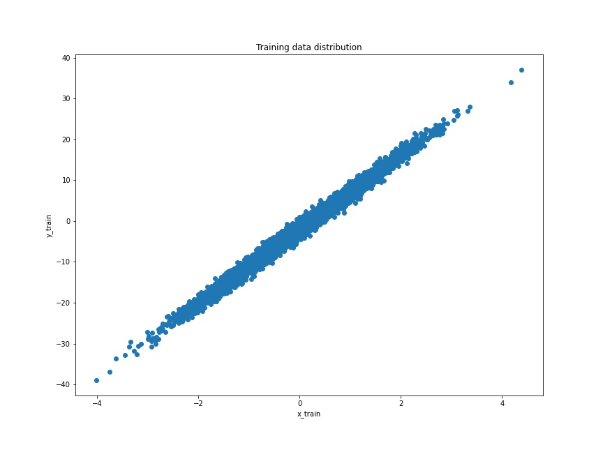
As we can see, the distribution is pretty linear and our linear regression model might be able to learn it pretty easily. Our main objective is to learn about the concept of linear regression using the TensorFlow GradientTape API. So, it does not matter much whether our data distribution is difficult or easy to learn.

Initialize Random Weight and Bias Values

The next block contains the code for initializing random values for weight and bias.

# random initial values for weights
W = tf.Variable(np.random.randn())
B = tf.Variable(np.random.randn())
print(W)
print(B)

<tf.Variable 'Variable:0' shape=() dtype=float32, numpy=1.4115247>
<tf.Variable 'Variable:0' shape=() dtype=float32, numpy=-0.7143893>

Our W and B values have been initialized to values very close to zero to start out with. With each training epoch, we will keep updating these weight and bias values so that they can actually start to match the initial m and c, that is, 9 and -2 respectively.

It is also important to note that W and B should be tf.Variable and not tf.contant tensors. This ensures that the values can be changed and tracked during runtime operations.

A Few Helper Functions

In this section, we will write a few helper functions that will make our work easier while running the training loop. These are mainly functions to calculate the predictions, the loss, and the gradients of W and B.

Let’s start with the prediction function.

def pred(x, W, B):
    """
    calculate y_hat = m*x + c with learned weights and biases.
    y_hat is the prediction
    """
    y_hat = W*x + B
    return y_hat

The pred() function accepts the training data points x, the weights W, and the bias B as the parameters. Then we calculate the values of predicted y using the formula y_hat = W*x + B and simply return the predicted value. This predicted y_hat value is the \(\hat{y}\) that we discussed earlier.

Next, the function to calculate the loss value, which is the Mean Squared Error (MSE) loss.

def loss(x, y, W, B):
    """
    Mean squared error loss function
    """
    prediction = pred(x, W, B)
    squared_error = tf.square(prediction - y)
    # finally calculate the MSE (Mean Sqaured Error)
    mse = tf.reduce_mean(squared_error)
    return mse

The loss() function accepts x, the original dependent variable y, the weight W, and the bias B.

• First, we call the pred function to get the prediction, that is, \(\hat{y}\).
• Then we use the tf.square() function to get the squared difference between the prediction and actual y.
• Finally, we calculate the MSE using tf.reduce_mean() function and return the value.

The final helper function is to calculate the gradients of W and B.

def calculate_gradient(x, y, W, B):
    """
    Calculate the derivative of the loss
    """
    with tf.GradientTape() as tape:
        loss_value = loss(x, y, W, B)
        
    w_grad, b_grad = tape.gradient(loss_value, [W, B])
    return w_grad, b_grad

The calculate_gradient() function also accepts x, the original dependent variable y, the weight W, and the bias B as the parameters.

• We call the loss() function within the tf.GradientTape() context and store it in loss_value. This ensures that all the operations on loss_value are tracked and recorded so that we use it to calculate the gradients.
• Next, we use gradient() function to get the gradients of W and B as w_grad and b_grad using the loss value. Then we return the two gradient values.

This is all we need for the helper functions. Now, let’s move on to the actual training part.

Training

As defined at the beginning of the coding section, we will train for 3000 epochs. The following are the steps that we will follow.

For each training epoch:

• We will calculate the y_hat using training data point x, W, and B.
• Then we will calculate the MSE using actual y and y_hat.
• Then the gradients, w_grad and b_grad get calculated.
• We compute the change that we want to subtract from current W and B by multiplying the learning rate with w_grad and b_grad.
• Finally, we update the values of W and B to new ones.

The following code block contains the code which will make things clearer.

for epoch in range(num_epochs):
    w_grad, b_grad = calculate_gradient(x_train, y_train, W, B)
    
    dW, dB = w_grad * learning_rate, b_grad * learning_rate
    
    W.assign_sub(dW)
    B.assign_sub(dB)
    
    if epoch % 10 == 0:
        print(f"Epoch: {epoch}, loss {loss(x_train, y_train, W, B):.3f}")

In the above block:

• dW and dB are the change in W and B that we get by multiplying the learning rate with the respective gradients.
• W.assign_sub(dW) and B.assign_sub(dB) are the two operations where we subtract the change and assign the new values for W and B. This is where the weight and bias get updated.
• Then we print the loss values after every 10 epochs.

Running the above code block will give output similar to the following.

Epoch: 0, loss 51.641
Epoch: 10, loss 49.641
Epoch: 20, loss 47.720
Epoch: 30, loss 45.875
Epoch: 40, loss 44.103
Epoch: 50, loss 42.401
Epoch: 60, loss 40.766
Epoch: 70, loss 39.195
Epoch: 80, loss 37.687
Epoch: 90, loss 36.238
Epoch: 100, loss 34.847
...
Epoch: 2970, loss 1.004
Epoch: 2980, loss 1.004
Epoch: 2990, loss 1.004

The loss started pretty high, around 51.6. But by the end of the training, it has dropped almost near to 1. This shows that our training is working and W and B are getting properly updated with each epoch.

Check the Final W and B Values

Let’s check the final W and B values after the training. If the learning has actually happened, then they should be very near to the initial m and c, which were 9 and -2 respectively.

# check whether we get the desired `m` and `c` or not
print(f"Learned W: {W.numpy()}, learned B: {B.numpy()}")

Learned W: 8.967373847961426, learned B: -2.011993169784546

As we can see, W is 8.967 and B is -2.011. This looks pretty good.

Testing on the Test Set

If you remember, then we also have one test set, that is, x_test and y_test. We will try to predict \(\hat{y}\) on this set. But before that, let’s check out the distribution of the test set.

# plot the test set
plt.figure(figsize=(12, 9))
plt.scatter(x_test, y_test)
plt.xlabel('x_test')
plt.ylabel('y_test')
plt.title('Test data distribution')
plt.savefig('test_data.jpg')

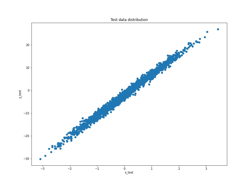
The test scatter plot looks almost similar to the training scatter plot as the data is from the same distribution only.

Check the Final Loss on the Test Set

Let’s see what we get when trying to calculate the final loss on the test set.

test_loss = loss(x_test, y_test, W, B)
print(f"Test loss: {test_loss:.3f}")

Test loss: 0.928

We are getting the loss value as 0.928 which is very near to what we got for the training data by the end of the training epochs.

Finally, let’s calculate the \(\hat{y}\) on the test data and see if we are actually able to fit on the test data or not.

# predicted y on on the test set
y_test_predicted = W.numpy()*x_test + B.numpy()
# plot the predicted y values on the test data distribution
plt.figure(figsize=(12, 9))
plt.plot(x_test, y_test_predicted, c='red')
plt.scatter(x_test, y_test)
plt.xlabel('x_test')
plt.ylabel('y_test')
plt.title('Test data distribution and predicted y plot')
plt.savefig('test_data_with_predicted_y_values.jpg')

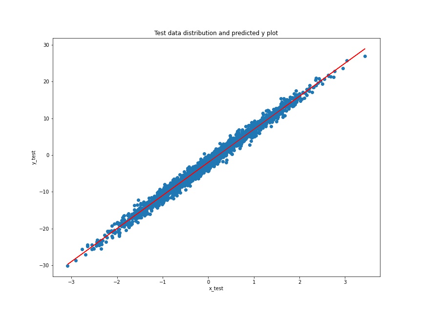
The predicted plot (red line) looks pretty good actually. It is almost able to fit in the test data. Looks like our linear regression model has found very optimized values W and B. Although it must be easy for the model to predict the values as the distribution of test data is the same as the training data. Still, it is good enough, for now, to learn the concepts of simple linear regression using TensorFlow’s GradientTape API.

With this, we have completed the coding part of this tutorial.

Summary and Conclusion

In this tutorial, we covered linear regression using TensorFlow’s GradientTape API. We did very basic training on a simple dummy dataset. We used a simple linear regression model with only one dependent feature vector. And we tried to predict the dependent values while trying to optimize the weight and bias values. But this should be enough to get someone started with the concepts if using the GradientTape API on other complex datasets as well. I hope that you learned something new in this tutorial.

If you have any doubts, thoughts, or suggestions, then please leave them in the comment section. I will surely address them.

You can contact me using the Contact section. You can also find me on LinkedIn, and Twitter.