Transfer Learning using TensorFlow

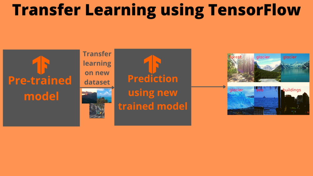
Whenever any researcher publishes a new deep learning model for image classification, they train it on the ImageNet dataset. There are two reasons for this. One, the ImageNet dataset is a widely accepted image classification data to compare new deep learning models. Secondly, others who do not have as much compute power to train the models themselves can use the pre-trained weights. But along with using the pre-trained weights, we can also use the model for transfer learning on our own dataset. And that is exactly what we will be doing in this tutorial. Here, you will learn about Transfer Learning using TensorFlow.

This post is the eighth post in the series, Getting Started with TensorFlow.

• Introduction to Tensors in TensorFlow.
• Basics of TensorFlow GradientTape.
• Linear Regression using TensorFlow GradientTape.
• Training Your First Neural Network in TensorFlow.
• Convolutional Neural Network in TensorFlow.
• Image Classification using TensorFlow on Custom Dataset.
• Image Classification using TensorFlow Pretrained Models.
• Transfer Learning using TensorFlow.

In the previous post of the series, we saw how to use pre-trained models in TensorFlow to carry out image classification.

In this tutorial, we will take one such pre-trained model and try transfer learning on a fairly large image dataset. Using transfer learning, we should get much better results than training a model from scratch.

So, what are we going to cover in this tutorial?

• We will start off with exploring the dataset that we will use. That is the Intel Image Classification dataset from Kaggle.
• Then we will write the code to load an ImageNet pre-trained model in TensorFlow.
  • We will use the MobileNetV2 model for transfer learning using TensorFlow.
• We will train the model on our own dataset and save the trained model as well.
• Then we will load the trained model and carry out predictions on unseen images.
• Finally, we will end the tutorial with a few takeaways and a short summary.

The Intel Image Classification Dataset

We will use the Intel Image Classification dataset for transfer learning using TensorFlow.

The Intel Image Classification dataset available on Kaggle is a great one to experiment with for transfer learning.

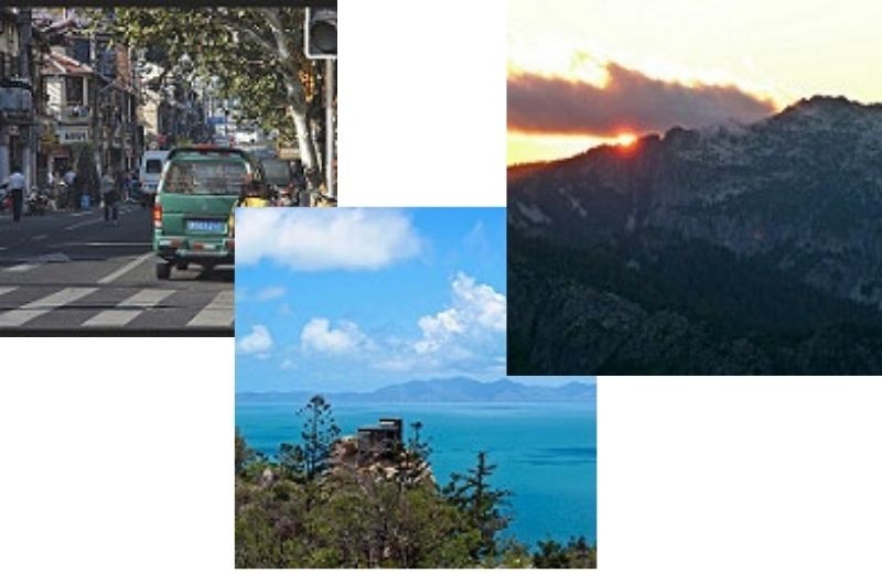
It has 25000 images and 6 classes in total. The classes are:

• buildings: class 0.
• forest: class 1.
• glacier: class 2.
• moutain: class 3.
• sea: class 4.
• street: class 5.

You can go ahead and download the dataset for now. We will see how to structure the directory a bit further on into the post.

There are already three splits available in the dataset. The training split has 14000 images, the test split has 3000 images, and there is a prediction split as well.

We will use the train split as training data and the test split as validation data while training the neural network. The prediction split does not contain any ground truth labels.

├── intel-image-classification
│   ├── seg_pred
│   │   └── seg_pred
│   ├── seg_test
│   │   └── seg_test
│   │       ├── buildings
│   │       ├── forest
│   │       ├── glacier
│   │       ├── mountain
│   │       ├── sea
│   │       └── street
│   └── seg_train
│       └── seg_train
│           ├── buildings
│           ├── forest
│           ├── glacier
│           ├── mountain
│           ├── sea
│           └── street

Above is the folder structure of the dataset. We can see the seg_train and seg_test have the images inside subfolders having the respective class names. This makes our work easier as we can directly use TensorFlow’s flow_from_directory function to prepare the dataset.

One other thing to note here, the seg_pred folder contains images without ground truths. And it has around 7000 images. We can use the images as unseen test images after training. We will not run the test on all 7000 images, but only a selected few.

The Directory Structure

Let’s take a look at the directory structure for this project.

├── checkpoints
│   └── final_model
│       ├── assets
│       ├── variables
│       │   ├── variables.data-00000-of-00001
│       │   └── variables.index
│       ├── keras_metadata.pb
│       └── saved_model.pb
├── input
│   ├── intel-image-classification
│   │   ├── seg_pred
│   │   │   └── seg_pred [7301 entries exceeds filelimit, not opening dir]
│   │   ├── seg_test
│   │   │   └── seg_test
│   │   │       ├── buildings [437 entries exceeds filelimit, not opening dir]
│   │   │       ├── forest [474 entries exceeds filelimit, not opening dir]
│   │   │       ├── glacier [553 entries exceeds filelimit, not opening dir]
│   │   │       ├── mountain [525 entries exceeds filelimit, not opening dir]
│   │   │       ├── sea [510 entries exceeds filelimit, not opening dir]
│   │   │       └── street [501 entries exceeds filelimit, not opening dir]
│   │   └── seg_train
│   │       └── seg_train
│   │           ├── buildings [2191 entries exceeds filelimit, not opening dir]
│   │           ├── forest [2271 entries exceeds filelimit, not opening dir]
│   │           ├── glacier [2404 entries exceeds filelimit, not opening dir]
│   │           ├── mountain [2512 entries exceeds filelimit, not opening dir]
│   │           ├── sea [2274 entries exceeds filelimit, not opening dir]
│   │           └── street [2382 entries exceeds filelimit, not opening dir]
├── outputs [13 entries exceeds filelimit, not opening dir]
├── intel_image_classification_transfer_learning.ipynb
└── prediction.ipynb

Okay, these might look like a lot of files and directories but don’t panic, let’s go through them together.

• In the input folder, we have the intel-image-classification dataset folder which we have already seen in the previous section.
• The checkpoints folder will contain the saved model files after we complete training the neural network model.
• The outputs folder will hold any images, accuracy and loss plots that we will generate while executing the code.
• Then we have two Jupyter Notebooks. The intel_image_classification_transfer_learning.ipynb notebook contains code to train the neural network on the dataset. Finally, the prediction.ipynb notebook contains the code for carrying out inference on the seg_pred images using the trained model.

Be sure to explore the directories and data a bit more on your own before moving on to the next section.

The MobileNetV2 Neural Network Model

For this project, we will use the MobileNetV2 neural network model as the pre-trained model.

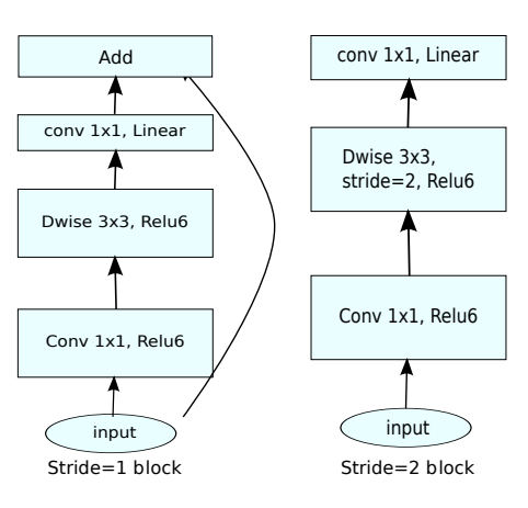
TensorFlow already provides a version of the model which has been pre-trained on the large ImageNet dataset. This means that the model has learned a lot of general image features. We can use these features to our benefit and train our neural network as well.

We will:

• Load the pre-trained MobileNetV2 model.
• Remove the 1000 class classification head that is present for the ImageNet classification.
• Add our own Dense layer for 6 class classification as the new head.
• And carry out the classification training.

Along with that, we will also freeze the weights in the MobileNetV2 layers. This means that no backpropagation will be performed to adjust the frozen weights. This will shorten the training time as only the only layer that is learnable is the Dense layer that we add at the end.

Transfer Learning using TensorFlow

From here onward, we will start writing the code for this tutorial. First, we will train our neural network model and save it to disk. Then we will carry out the predictions using the trained model.

All the code that we will write for training will go into the intel_image_classification_transfer_learning.ipynb notebook. The main reason for using Jupyter Notebooks for this tutorial is that it helps to visualize the outputs as soon as we execute the cell. So, it will be easier to understand the concepts.

Let’s start with the import statements.

import numpy as np
import pandas as pd
import matplotlib.pyplot as plt
import os
import tensorflow as tf
import matplotlib

matplotlib.style.use('ggplot')

The above code block imports the TensorFlow library along with all the other packages that we need.

Prepare the Dataset

Now, we will prepare the dataset. This includes:

• Visualizing a few of the images along with the ground truth labels from the training set.
• And preparing the training and validation data generators.

First, let’s define a list that contains all the class label names that we have in the dataset.

# define all the labels in a list
# will use later to visualize the images along with the proper labels
labels = ['buildings', 'forest', 'glacier', 'mountain', 
          'sea', 'street']

The labels list contains all the class names. Note that this corresponds to the folder names for each of the classes. Each of the folders contains the images corresponding to that class.

Visualize a Few Images

We will visualize one image from each of the classes. We already have the class from the above code block. So, we can access the respective folders using those class names, read an image from the folder, and display it. The following block contains the code for that.

TRAIN_PATH = 'input/intel-image-classification/seg_train/seg_train'
plt.figure(figsize=(12, 9))
for i, label in enumerate(labels):
    plt.subplot(2, 3, i+1)
    all_images = os.listdir(f"{TRAIN_PATH}/{label}/")
    image = plt.imread(f"{TRAIN_PATH}/{label}/{all_images[i]}")
    plt.imshow(image)
    plt.axis('off')
    plt.title(labels[i])
    plt.savefig('outputs/intel-images.png')
plt.show()

We define the TRAIN_PATH string that stores the path to the training image folders. Then we just iterate over the labels list and store all the image paths from that class folder in the all_images list. After that, we read the image and visualize it using Matplotlib.

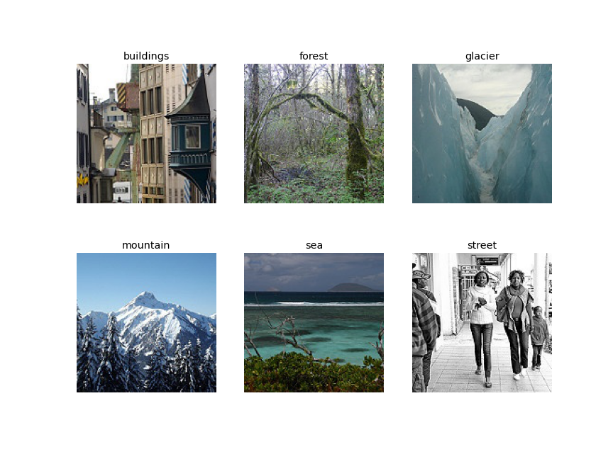
We can see images from each class in the above figure. This gives us a good idea of what kind of images there are in the dataset.

Prepare the Data Generators

Now, it’s time to prepare the training and validation data generators that will sample the images while we train the neural network.

For that, we need a few things which the following code block contains.

# define the image shape to resize to
IMAGE_SHAPE = (224, 224)
# train folder path
TRAINING_DATA_DIR = 'input/intel-image-classification/seg_train/seg_train'
# validataion folder path
VALID_DATA_DIR = 'input/intel-image-classification/seg_test/seg_test'

• IMAGE_SHAPE is the image dimension we want the images to resize to. Here, we want to resize the images to 224×224 dimension.
• TRAIN_DATA_DIR is the path to the folder that contains all the training class subfolders.
• Similarly, VALID_DATA_DIR is the path that contains all the validation class subfolders.

The next code block contains the code to prepare the data generators.

# data generator defining the image preprocessing
# we are only scaling the pixels here, not data augmentation
datagen = tf.keras.preprocessing.image.ImageDataGenerator(
    rescale=1./255
)

# define the train data generator
train_generator = datagen.flow_from_directory(
    TRAINING_DATA_DIR,
    shuffle=True,
    target_size=IMAGE_SHAPE,
)

# define the validation data generator
valid_generator = datagen.flow_from_directory(
    VALID_DATA_DIR,
    shuffle=False,
    target_size=IMAGE_SHAPE,
)

Let’s go through the code in the above block.

• datagen defines the image preprocessing that we want to carry out. Here, we are only rescaling the image pixels so that they will range between 0 and 1. We can also provide the image data augmentations of our choice here, but we are skipping that part to keep things simple.
• The train_generator uses the the datagen defined just above. It has a flow_from_directory function that takes the training class subfolders path. Along with that, we are shuffling the training data and resizing the images to 224×224 dimension.
• We use a similar approach to prepare the validation data generator, that is valid_generator.

By now, all our data preparation steps are complete. Executing the above code will give the following output.

Found 14034 images belonging to 6 classes.
Found 3000 images belonging to 6 classes.

This indicates that we have 14034 images for training and 3000 images for validation.

Prepare the Neural Network Model

As discussed earlier, we will use a pre-trained MobileNetV2 model as the base network.

Prepare the MobileNetV2 Base Network

For transfer learning, we need a pre-trained model in TensorFlow.

TensorFlow provides the keras.applications module to easily load many classification models that have been pre-trained on the ImageNet dataset. And MobileNetV2 is one of them.

def build_base_model(input_shape=(224, 224, 3)):
    """
    This function loads the pre-trained MobileNetV2 model.
    It has been trained on the ImageNet dataset and we will
    use the pre-trained weights.
    
    Args:
    input_shape: input shape of images
    """
    base_model = tf.keras.applications.MobileNetV2(
        input_shape=input_shape,
        include_top=False, # we don't need the model head, will add our own
        weights='imagenet'
    )
    return base_model

In the above code block, we define the build_base_model() function that accepts the input_shape as a parameter. We need the shape of the image to properly initialize the base network.

Using tf.keras.applications we load the MobileNetV2 model which takes the following arguments:

• The input_shape as 224x224x3.
• include_top=False defining that we do not need the 1000 class classification head as we will define our classification layer later on.
• And weights='imagenet' indicating to load the pre-trained ImageNet weights.

Let’s execute the above function now.

base_model = build_base_model(input_shape=(224, 224, 3))

Now, base_model holds all the MobileNetV2 feature layers.

The next step is to freeze all the layers so that weights will not be fine-tuned. We can do that with just one line of code.

# freeze the base model parameters
# we will not train the weights again
base_model.trainable = False

print(base_model.summary())

The following is the truncated base network summary.

Model: "mobilenetv2_1.00_224"
__________________________________________________________________________________________________
Layer (type)                    Output Shape         Param #     Connected to                     
==================================================================================================
input_1 (InputLayer)            [(None, 224, 224, 3) 0                                            
__________________________________________________________________________________________________
Conv1 (Conv2D)                  (None, 112, 112, 32) 864         input_1[0][0]                    
__________________________________________________________________________________________________
bn_Conv1 (BatchNormalization)   (None, 112, 112, 32) 128         Conv1[0][0]                      
__________________________________________________________________________________________________
Conv1_relu (ReLU)               (None, 112, 112, 32) 0           bn_Conv1[0][0] 
...
__________________________________________________________________________________________________
Conv_1 (Conv2D)                 (None, 7, 7, 1280)   409600      block_16_project_BN[0][0]        
__________________________________________________________________________________________________
Conv_1_bn (BatchNormalization)  (None, 7, 7, 1280)   5120        Conv_1[0][0]                     
__________________________________________________________________________________________________
out_relu (ReLU)                 (None, 7, 7, 1280)   0           Conv_1_bn[0][0]                  
==================================================================================================
Total params: 2,257,984
Trainable params: 0
Non-trainable params: 2,257,984
__________________________________________________________________________________________________
None

A few things to note here:

• The final convolutional layer has a 1280 output channels.
• There are a total of 2,257,984 parameters. But taking a closer look indicates that none of them are trainable as we have already frozen all the layers.

Add the Classification Layer

The final step to prepare the complete neural network model is to add the classification head.

# add classification layer on top and get the final model
def get_final_model(num_classes, base_model):
    """
    This function returns the final model after adding the classification
    head to the MobileNetV2 backbone. 
    
    Args:
    num_classes: number of classes in the dataset
    base_model: the backbone model
    """
    inputs = tf.keras.Input(shape=(224, 224, 3))
    # next layer is the input to the model, not to be trained
    x = base_model(inputs, training=False)
    x = tf.keras.layers.GlobalAveragePooling2D()(x)
    # the final `Dense` layer with the number of classes
    outputs = tf.keras.layers.Dense(num_classes)(x)
    # the final model
    model = tf.keras.Model(inputs, outputs)
    return model

model = get_final_model(num_classes=6, base_model=base_model)
print(model.summary())

The get_final_model() accepts the number of classes and base MobileNetV2 model as parameters.

First, we need to pass the inputs through the base_model. Do observe that we are passing the training argument as False for the inputs. This means that we do not want the inputs to be trainable. Then we add the GlobalAveragePooling2D layer to get the 2D outputs where the number of units will be equal to the previous layer’s channels. For the final layer, we add the classification head using Dense where the output units are equal to the number of classes. Finally, we prepare the model using tf.keras.model.

Following is the model summary.

Model: "model"
_________________________________________________________________
Layer (type)                 Output Shape              Param #   
=================================================================
input_2 (InputLayer)         [(None, 224, 224, 3)]     0         
_________________________________________________________________
mobilenetv2_1.00_224 (Functi (None, 7, 7, 1280)        2257984   
_________________________________________________________________
global_average_pooling2d (Gl (None, 1280)              0         
_________________________________________________________________
dense (Dense)                (None, 6)                 7686      
=================================================================
Total params: 2,265,670
Trainable params: 7,686
Non-trainable params: 2,257,984
_________________________________________________________________
None

We can see the input layer with 0 trainable parameters. Then we have the MobileNetV2 as the feature extractor layer followed by the GlobalAveragePooling2D. The final Dense layer has 7686 parameters which are the only trainable parameters in the whole model.

Next, let’s compile the model.

model.compile(
    # very big LR can throw off the training, so using a small LR
    optimizer=tf.keras.optimizers.Adam(lr=0.0001), 
    loss=tf.keras.losses.CategoricalCrossentropy(from_logits=True),
    metrics=['accuracy']
)

The learning rate is 0.0001 as a very big learning rate can diverge the training process. This mostly happens when using a pre-trained model. The loss function is Categorical Cross-Entropy. We are using accuracy as the metric.

Training

We will train for 10 epochs with a batch size of 32. If you face the OOM (Out Of Memory) error, then please reduce the batch size to 16 or 8.

EPOCHS = 10
BATCH_SIZE = 32
history = model.fit(train_generator,
                      steps_per_epoch=train_generator.samples // BATCH_SIZE,
                      epochs=EPOCHS,
                      validation_data=valid_generator,
                      validation_steps= valid_generator.samples // BATCH_SIZE,
                      verbose=1
                     )

If you want to get the details of all the arguments we pass to the fit(), then please take a look at this post here where we train a convolutional neural network from scratch.

The following is the out from the training.

Epoch 1/10
438/438 [==============================] - 99s 159ms/step - loss: 0.8102 - accuracy: 0.7187 - val_loss: 0.4506 - val_accuracy: 0.8599
Epoch 2/10
438/438 [==============================] - 118s 269ms/step - loss: 0.3779 - accuracy: 0.8801 - val_loss: 0.3382 - val_accuracy: 0.8841
Epoch 3/10
438/438 [==============================] - 31s 70ms/step - loss: 0.3116 - accuracy: 0.8962 - val_loss: 0.2970 - val_accuracy: 0.8921
Epoch 4/10
438/438 [==============================] - 31s 70ms/step - loss: 0.2819 - accuracy: 0.9052 - val_loss: 0.2797 - val_accuracy: 0.8948
Epoch 5/10
438/438 [==============================] - 31s 70ms/step - loss: 0.2657 - accuracy: 0.9090 - val_loss: 0.2669 - val_accuracy: 0.8952
Epoch 6/10
438/438 [==============================] - 31s 71ms/step - loss: 0.2539 - accuracy: 0.9124 - val_loss: 0.2586 - val_accuracy: 0.8999
Epoch 7/10
438/438 [==============================] - 31s 71ms/step - loss: 0.2445 - accuracy: 0.9150 - val_loss: 0.2524 - val_accuracy: 0.9002
Epoch 8/10
438/438 [==============================] - 31s 71ms/step - loss: 0.2378 - accuracy: 0.9157 - val_loss: 0.2487 - val_accuracy: 0.9012
Epoch 9/10
438/438 [==============================] - 31s 72ms/step - loss: 0.2311 - accuracy: 0.9182 - val_loss: 0.2455 - val_accuracy: 0.8989
Epoch 10/10
438/438 [==============================] - 31s 70ms/step - loss: 0.2254 - accuracy: 0.9217 - val_loss: 0.2430 - val_accuracy: 0.9015

By the end of 10 epochs, we have a validation loss of 0.2430 and validation accuracy of 90.15%. This seems pretty good considering that we have trained only the classification head while keeping the base layer frozen.

And now, let’s take a look at the loss and accuracy plots.

train_loss = history.history['loss']
train_acc = history.history['accuracy']
valid_loss = history.history['val_loss']
valid_acc = history.history['val_accuracy']

def save_plots(train_acc, valid_acc, train_loss, valid_loss):
    """
    Function to save the loss and accuracy plots to disk.
    """
    # accuracy plots
    plt.figure(figsize=(12, 9))
    plt.plot(
        train_acc, color='green', linestyle='-', 
        label='train accuracy'
    )
    plt.plot(
        valid_acc, color='blue', linestyle='-', 
        label='validataion accuracy'
    )
    plt.xlabel('Epochs')
    plt.ylabel('Accuracy')
    plt.legend()
    plt.savefig('outputs/accuracy.png')
    plt.show()
    # loss plots
    plt.figure(figsize=(12, 9))
    plt.plot(
        train_loss, color='orange', linestyle='-', 
        label='train loss'
    )
    plt.plot(
        valid_loss, color='red', linestyle='-', 
        label='validataion loss'
    )
    plt.xlabel('Epochs')
    plt.ylabel('Loss')
    plt.legend()
    plt.savefig('outputs/loss.png')
    plt.show()

save_plots(train_acc, valid_acc, train_loss, valid_loss)

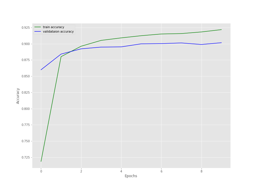
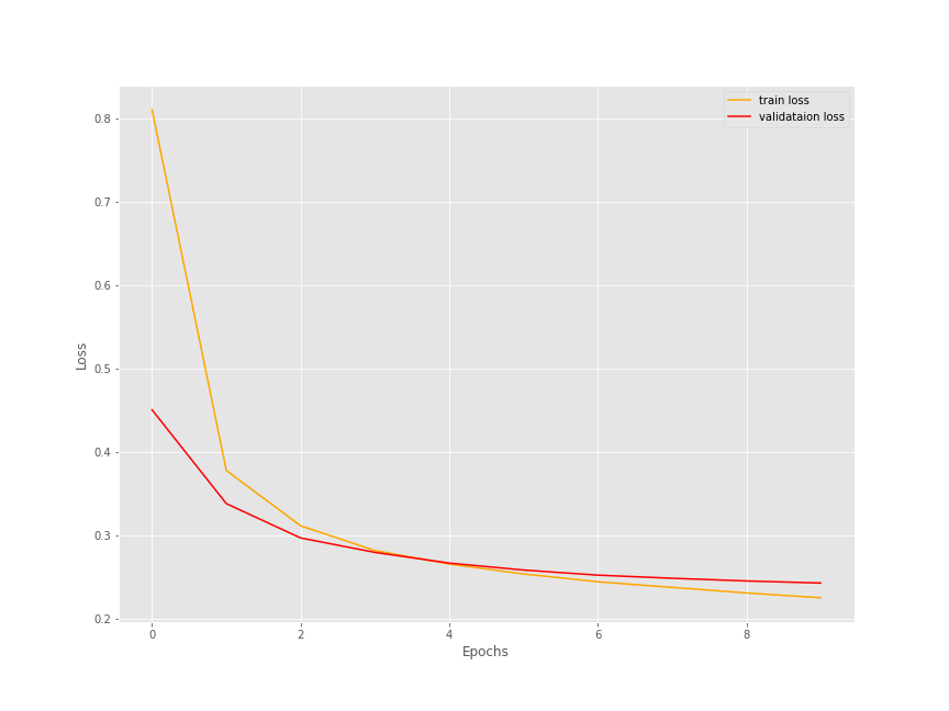
The training accuracy was still increasing but the validation accuracy seems to be starting to plateau a bit. For the loss, both training and validation loss seems to be decreasing even at 10 epochs. Still, it looks like 10 epochs are just perfect for now.

Save the Entire Model

There is just one more step before we move on to the inference notebook. We need to save the trained model. We will use the save() function to save the entire model so that we can resume training if we want to.

# save the final model
model.save('checkpoints/final_model')

All the model files will be saved in the final_model folder inside the checkpoints folder.

This completes the training part of this tutorial. We are ready to move on to the inference notebook.

Inference Using the Trained Model

Our transfer learning phase is complete as we have trained our model using TensorFlow.

This is going to be a very short notebook. We will load the saved model from the disk and carry out inference on some of the images inside the input/intel-image-classification/seg_pred/seg_pred folder.

All the code that we will write here will go into the prediction.ipynb notebook.

First, we import all the required libraries and modules and create a list containing all the class names.

import tensorflow as tf
import glob as glob
import cv2
import matplotlib.pyplot as plt
import numpy as np

# prepare label names 
labels = ['buildings', 'forest', 'glacier', 'mountain', 
          'sea', 'street']

Load the Trained Model

We can easily load the trained model using tf.keras.models.load_model.

model = tf.keras.models.load_model('checkpoints/final_model')

Carry Out the Inference

We need the image paths to read them. Let’s get all the paths using the glob module and store in a image_paths list.

# get all the image paths
image_paths = glob.glob('input/intel-image-classification/seg_pred/seg_pred/*')
print(f"Number of images for prediction: {len(image_paths)}")

The above code will give the following output.

Number of images for prediction: 7301

There are 7301 images in the prediction folder. We cannot carry out inference on all these images.

Let’s check the prediction on 10 images.

for i in range(10):
    image = cv2.imread(image_paths[i])
    orig_image = image.copy()
    image = cv2.cvtColor(image, cv2.COLOR_BGR2RGB)
    image = cv2.resize(image, (224, 224))
    image = image / 255.
    image = np.expand_dims(image, axis=0)
    predictions = model(image)
    label = labels[np.argmax(predictions)]
    cv2.putText(orig_image, label, (10, 25), cv2.FONT_HERSHEY_SIMPLEX, 
                0.7, (0, 0, 255), 1, cv2.LINE_AA)
    plt.imshow(orig_image[:, :, ::-1])
    plt.show()
    cv2.imwrite(f"outputs/pred_{i}.png", orig_image)
    print(label)
    print('-'*50) 

The steps are pretty simple.

• We read the image using cv2 and keep a copy of the original image to use later on for OpenCV annotations, such as writing the class name on top of the image.
• For the image, which we use for prediction, we convert the color format from BGR to RGB, resize it to 224×224 dimension, and scale the pixel values. After that we add a batch dimension to make the final shape as 1x224x224x3.
• Then we pass the image through the model and get the predictions. We get the final label by mapping the index of the highest value in predictions to the labels list.
• Then we show the image in the output cell and save the resulting output in the outputs folder.

Here are a few of the results.

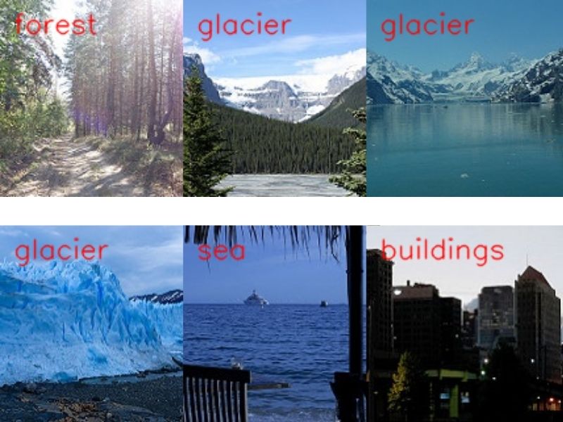
Wow! looks like the model is predicting really well. It has predicted all the images correctly.

A Few Takeaways

• We saw that the trained model is predicting really well. Then why not use the model to create a larger training set by running inference on the prediction set and storing the images in the trainig folder? Surely, we will have to double check each image prediction, still it will be faster than manual annotation.
• You can even train a larger model after creating a larger training set.
• Try models such a ResNet18, ResNet34, and Inception networks for transfer learning using TensorFlow. Let us know the results in the comment section.

Summary and Conclusion

In this tutorial, you learned how to use transfer learning to quickly train an image classifier in TensorFlow with high accuracy. We used the MobileNetV2 as the base model and added our own classification head. We also discussed how to use the trained model to enlarge our training set by creating automatic labels. I hope that you learned something new from this tutorial.

If you have any doubts, thoughts, or suggestions, then please leave them in the comment section. I will surely address them.

You can contact me using the Contact section. You can also find me on LinkedIn, and Twitter.