
In this tutorial, you will learn how to train a deep learning model on a custom dataset using TensorFlow. In particular, you will learn how to do image classification on a custom dataset using TensorFlow.
This post is the sixth in the series, Getting Started with TensorFlow.
- Introduction to Tensors in TensorFlow.
- Basics of TensorFlow GradientTape.
- Linear Regression using TensorFlow GradientTape.
- Training Your First Neural Network in TensorFlow.
- Convolutional Neural Network in TensorFlow.
- Image Classification using TensorFlow on Custom Dataset.
After going through this tutorial, you will have the knowledge to train convolutional neural networks for image classification tasks using TensorFlow on your own dataset.
We will be covering the following topics in this tutorial.
- We will start with exploring the dataset that we will use. That is, the 10 Monkey Species dataset available on Kaggle.
- Then we will get to know the directory structure for this tutorial.
- Following that, we will start with the coding part.
- We will prepare our dataset.
- Build our convolutional neural network model.
- Train the model and analyze the results.
- Finally, we will cover a few takeways from the this project before concluding the tutorial.
Let’s jump into the tutorial without any further delay.
Exploring the Dataset
We will use the 10 Monkey Species dataset from Kaggle. It is a good dataset to learn image classification using TensorFlow for custom datasets. The dataset contains images for 10 different species of monkeys.
The following image shows all the information for the dataset. This contains the labels, the Latin names for the monkey species, the common names, and the number of training and validation images for each class.
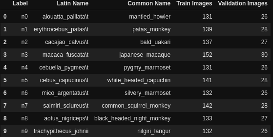
As you can see we have 10 classes in total. The n0 to n9 are the folder names for each of the monkey classes which contain the images for that particular species.
And the following is the folder structure after you download and extract the entire dataset.
├── training
│   └── training
│       ├── n0 [105 entries exceeds filelimit, not opening dir]
│       ├── n1 [111 entries exceeds filelimit, not opening dir]
│       ├── n2 [110 entries exceeds filelimit, not opening dir]
│       ├── n3 [122 entries exceeds filelimit, not opening dir]
│       ├── n4 [105 entries exceeds filelimit, not opening dir]
│       ├── n5 [113 entries exceeds filelimit, not opening dir]
│       ├── n6 [106 entries exceeds filelimit, not opening dir]
│       ├── n7 [114 entries exceeds filelimit, not opening dir]
│       ├── n8 [106 entries exceeds filelimit, not opening dir]
│       └── n9 [106 entries exceeds filelimit, not opening dir]
├── validation
│   └── validation
│       ├── n0 [26 entries exceeds filelimit, not opening dir]
│       ├── n1 [28 entries exceeds filelimit, not opening dir]
│       ├── n2 [27 entries exceeds filelimit, not opening dir]
│       ├── n3 [30 entries exceeds filelimit, not opening dir]
│       ├── n4 [26 entries exceeds filelimit, not opening dir]
│       ├── n5 [28 entries exceeds filelimit, not opening dir]
│       ├── n6 [26 entries exceeds filelimit, not opening dir]
│       ├── n7 [28 entries exceeds filelimit, not opening dir]
│       ├── n8 [27 entries exceeds filelimit, not opening dir]
│       └── n9 [26 entries exceeds filelimit, not opening dir]
└── monkey_labels.txt
As you can see, we have the training and validation folders. And these again contain another training and validation folder each. After that, each of the folders contains the n0 to n9 folders which will act as the labels and they contain the respective images for each class. We also have the monkey_labels.txt which contains all the information about the dataset that we just saw above.
To finish off the exploration of the dataset, let’s visualize one image from each of the monkey species classes.
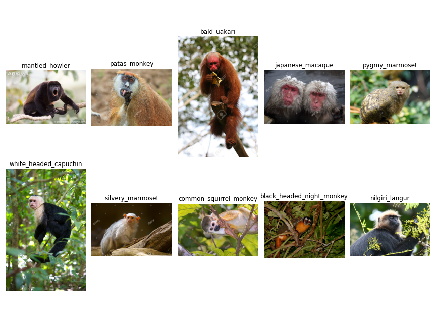
You may explore the dataset a bit more before jumping into the coding part. This will help you become more familiar with the data you are dealing with.
Also, if you download the source code for this tutorial, then you will find the code for the above image visualization in the eda.ipynb notebook.
Directory Structure
Let’s take a look at the directory structure that we will follow for this project.
├── input
│   ├── training
│   │   └── training
│   │       ├── n0 [105 entries exceeds filelimit, not opening dir]
│   │       ├── n1 [111 entries exceeds filelimit, not opening dir]
│   │       ├── n2 [110 entries exceeds filelimit, not opening dir]
│   │       ├── n3 [122 entries exceeds filelimit, not opening dir]
│   │       ├── n4 [105 entries exceeds filelimit, not opening dir]
│   │       ├── n5 [113 entries exceeds filelimit, not opening dir]
│   │       ├── n6 [106 entries exceeds filelimit, not opening dir]
│   │       ├── n7 [114 entries exceeds filelimit, not opening dir]
│   │       ├── n8 [106 entries exceeds filelimit, not opening dir]
│   │       └── n9 [106 entries exceeds filelimit, not opening dir]
│   ├── validation
│   │   └── validation
│   │       ├── n0 [26 entries exceeds filelimit, not opening dir]
│   │       ├── n1 [28 entries exceeds filelimit, not opening dir]
│   │       ├── n2 [27 entries exceeds filelimit, not opening dir]
│   │       ├── n3 [30 entries exceeds filelimit, not opening dir]
│   │       ├── n4 [26 entries exceeds filelimit, not opening dir]
│   │       ├── n5 [28 entries exceeds filelimit, not opening dir]
│   │       ├── n6 [26 entries exceeds filelimit, not opening dir]
│   │       ├── n7 [28 entries exceeds filelimit, not opening dir]
│   │       ├── n8 [27 entries exceeds filelimit, not opening dir]
│   │       └── n9 [26 entries exceeds filelimit, not opening dir]
│   └── monkey_labels.txt
├── eda.ipynb
├── monkey-species-classification.ipynb
- First of all, we can see the
inputfolder which contains the data that we discussed above. - Then we have two Jupyter Notebooks. The
eda.ipynbcontains the code to explore the data a bit and visualize the image that we saw above. Themonkey-species-classification.ipynbNotebook contains the code for image classification using TensorFlow.
Along with the above files, the loss and accuracy plots will also be generated as we start executing the monkey-species-classification.ipynb Notebook.
From the next section onward, we will focus on the coding section of the tutorial.
Image Classification using TensorFlow
Let’s start with the coding part of the tutorial without any further delay. All of the code from here onward will go into the monkey-species-classification.ipynb notebook.
The following are the imports that we need along the way.
import matplotlib.pyplot as plt
import os
import tensorflow as tf
import matplotlib

matplotlib.style.use('ggplot')
We need matplotlib to plot the accuracy and loss graphs after the training.
Creating Data Generators for Training and Validation
Before we can begin our image classification training using TensorFlow, we need to prepare the training and validation data.
TensorFlow provides the ImageDataGenerator class that can handle the preprocessing of the images for us. And this class has a flow_from_directory function that handles the preparation of the training and validation data for us with ease. In fact, we do not even need to provide the number of classes we have in our dataset.
We just need to provide the path to the training and validation folders which contain the images of each class in their respective subfolders.
For example, our input folder has the following structure.
├── input
│   ├── training
│   │   └── training
│   │       ├── n0
│   │       ...
│   │       └── n9
│   ├── validation
│   │   └── validation
│   │       ├── n0
│   │       ...
│   │       └── n9
Above, n0 to n9 are the different class folders that contain the images. So, we just need to provide the path as input/training/training/ and input/validation/validation/ to the flow_from_directory function to prepare the training and validation data respectively.
Let’s take a look at the code, and things will become much more clear.
IMAGE_SHAPE = (224, 224)
TRAINING_DATA_DIR = 'input/training/training/'
VALID_DATA_DIR = 'input/validation/validation/'
We need to define the shape of the images that we want to train on. The images will be resized accordingly before being fed into the neural network. And we will be resizing the images to 224×224 size.
Then TRAINING_DATA_DIR and VALID_DATA_DIR hold the paths to the training and validation image class sub folders respectively.
Moving on to the next chunk of code.
datagen = tf.keras.preprocessing.image.ImageDataGenerator(
    rescale=1./255
)

train_generator = datagen.flow_from_directory(
    TRAINING_DATA_DIR,
    shuffle=True,
    target_size=IMAGE_SHAPE,
)

valid_generator = datagen.flow_from_directory(
    VALID_DATA_DIR,
    shuffle=False,
    target_size=IMAGE_SHAPE,
)
In the above code block:
- We initalize
datagenwithtf.keras.preprocessing.image.ImageDataGenerator. This takes in any image preprocessing and image augmentations that we want to apply to images. In our case, we are just normalizing the images to scale the pixels between 0 and 1. Take a look at the official docs to know what kind of augmentations we can provide. - Then
train_generatoruses theflow_from_directoryfunction. Here, we provide the training data directory path, keepshuffle=Trueand provide thetarget_sizeto resize the images. - We follow a similar approach to prepare the validation data that
valid_generatorholds.
After executing the above code cell, you will get the following output.
Found 1098 images belonging to 10 classes.
Found 272 images belonging to 10 classes.
This shows that we have 1089 images for training and 272 images for validation.
Build and Compile the Model
We will build a simple neural network model consisting of 2D Convolutional layers, 2D Max-Pooling layers, and Linear layers. And we will use the Sequential class to build the model.
def build_model(num_classes):
    model = tf.keras.Sequential([
    tf.keras.layers.Conv2D(filters=8, kernel_size=(3, 3), activation='relu',
                           input_shape=(224, 224, 3)),
    tf.keras.layers.MaxPooling2D(pool_size=(2, 2), strides=2),
    tf.keras.layers.Conv2D(filters=16, kernel_size=(3, 3), activation='relu'),
    tf.keras.layers.MaxPooling2D(pool_size=(2, 2), strides=2),
    tf.keras.layers.Conv2D(filters=32, kernel_size=(3, 3), activation='relu'),
    tf.keras.layers.MaxPooling2D(pool_size=(2, 2), strides=2),
    tf.keras.layers.Flatten(),
    tf.keras.layers.Dense(64, activation='relu'),
    tf.keras.layers.Dense(num_classes, activation='softmax')
    ])
    return model

model = build_model(num_classes=10)
- We define a
build_model()function which accepts the number of classes as parameter. - The first
Conv2Dlayer has 8filterswith 3×3kernel_sizeandreluactivation. Note that we need to provide theinput_shapehere and this should be the same as the size to which the images are being resized by theImageDataGenerator. It is followed by aMaxPooling2Dlayer with 2×2pool_sizeandstridesof 2. - We have two more such stackings of convolutional and max-pooling layers. Each time we increase the number of
filtersin the convolutional layer. - Then we
Flattenthe input before feeding the features to aDenselayer with 64 units. And the finalDenselayer has number of units similar tonum_classeswith softmax activation function. - Finally, we execute the
build_model()function by providingnum_classes=10as the argument.
Compile the Model
Let’s compile the model now.
model.compile(
    optimizer=tf.keras.optimizers.Adam(lr=0.0001),
    loss=tf.keras.losses.CategoricalCrossentropy(from_logits=True),
    metrics=['accuracy']
)

print(model.summary())
We are using the Adam optimizer with a learning rate of 0.0001. We are not using a very high learning rate as the training may get unstable. Using a too low learning rate might also lead the model to not converge to an optimal solution. Hopefully, our learning rate value will work considerably well.
For the loss function, we are using the Categorical Cross-Entropy loss. And our evaluation metric is accuracy.
Printing the model summary gives the following output.
Model: "sequential"
_________________________________________________________________
Layer (type)                 Output Shape              Param #
=================================================================
conv2d (Conv2D)              (None, 222, 222, 8)       224
_________________________________________________________________
max_pooling2d (MaxPooling2D) (None, 111, 111, 8)       0
_________________________________________________________________
conv2d_1 (Conv2D)            (None, 109, 109, 16)      1168
_________________________________________________________________
max_pooling2d_1 (MaxPooling2 (None, 54, 54, 16)        0
_________________________________________________________________
conv2d_2 (Conv2D)            (None, 52, 52, 32)        4640
_________________________________________________________________
max_pooling2d_2 (MaxPooling2 (None, 26, 26, 32)        0
_________________________________________________________________
flatten (Flatten)            (None, 21632)             0
_________________________________________________________________
dense (Dense)                (None, 64)                1384512
_________________________________________________________________
dense_1 (Dense)              (None, 10)                650
=================================================================
Total params: 1,391,194
Trainable params: 1,391,194
Non-trainable params: 0
_________________________________________________________________
None
Out model contains 1,391,194 trainable parameters. This is not very high and most probably the training will be fast enough even on a CPU.
Training the Image Classification Model using TensorFlow
As usual, we will use the fit() method to train the model and will have all the loss and accuracy values in the history object.
But the arguments for the fit() method are going to be a bit different than what we used in the previous posts for training in this Getting Started with TensorFlow series.
The following block contains the code. Let’s check that out and then get into the explanation part.
EPOCHS = 20
BATCH_SIZE = 32
history = model.fit(train_generator,
                    steps_per_epoch=train_generator.samples // BATCH_SIZE,
                    epochs=EPOCHS,
                    validation_data=valid_generator,
                    validation_steps= valid_generator.samples // BATCH_SIZE,
                    verbose=1
                    )
- First of all, we are training for 20 epochs and the batch size is 32. If you are getting Out Of Memory error, then try reducing the batch size to 16, or 8, and it will work out smoothly.
- Then we have the
fit()method. The first argument is thetrain_generatorthat will sample the training data and feed into the neural network. - Next we provide
steps_per_epochthat defines how to update the progress bar while training. Generally, number of training sampels divided by batch gives a good idea of the progress bar update. Even if we do not provide any value for this argument, then it will autoamtically take number of samples divided by the batch size. - Then we provide the
epochs, that is 20 in our case. - Then the
validation_dataand thevalidation_stepswhich is again number of validation samples divided by the batch size. - Finally, we provide
verbose=1to show the progress bar while training.
The following block shows the output of the entire training process.
Epoch 1/20
34/34 [==============================] - 82s 1s/step - loss: 2.2851 - accuracy: 0.1529 - val_loss: 2.2483 - val_accuracy: 0.1602
Epoch 2/20
34/34 [==============================] - 36s 1s/step - loss: 2.1699 - accuracy: 0.2205 - val_loss: 2.1186 - val_accuracy: 0.2344
Epoch 3/20
34/34 [==============================] - 34s 1s/step - loss: 2.0479 - accuracy: 0.2795 - val_loss: 2.0304 - val_accuracy: 0.2656
Epoch 4/20
34/34 [==============================] - 24s 720ms/step - loss: 1.9581 - accuracy: 0.3152 - val_loss: 1.9431 - val_accuracy: 0.3047
Epoch 5/20
34/34 [==============================] - 24s 723ms/step - loss: 1.8423 - accuracy: 0.3649 - val_loss: 1.9293 - val_accuracy: 0.3594
Epoch 6/20
34/34 [==============================] - 26s 778ms/step - loss: 1.7556 - accuracy: 0.3987 - val_loss: 1.8179 - val_accuracy: 0.3516
Epoch 7/20
34/34 [==============================] - 25s 738ms/step - loss: 1.6756 - accuracy: 0.4503 - val_loss: 1.7499 - val_accuracy: 0.4297
Epoch 8/20
34/34 [==============================] - 25s 729ms/step - loss: 1.5613 - accuracy: 0.5113 - val_loss: 1.7231 - val_accuracy: 0.4023
Epoch 9/20
34/34 [==============================] - 24s 719ms/step - loss: 1.4597 - accuracy: 0.5347 - val_loss: 1.6877 - val_accuracy: 0.4297
Epoch 10/20
34/34 [==============================] - 24s 703ms/step - loss: 1.4203 - accuracy: 0.5507 - val_loss: 1.6423 - val_accuracy: 0.4648
Epoch 11/20
34/34 [==============================] - 25s 740ms/step - loss: 1.3355 - accuracy: 0.5807 - val_loss: 1.5939 - val_accuracy: 0.4766
Epoch 12/20
34/34 [==============================] - 24s 715ms/step - loss: 1.2567 - accuracy: 0.6210 - val_loss: 1.6136 - val_accuracy: 0.4609
Epoch 13/20
34/34 [==============================] - 24s 725ms/step - loss: 1.2086 - accuracy: 0.6257 - val_loss: 1.5623 - val_accuracy: 0.4883
Epoch 14/20
34/34 [==============================] - 23s 680ms/step - loss: 1.1429 - accuracy: 0.6585 - val_loss: 1.5080 - val_accuracy: 0.4883
Epoch 15/20
34/34 [==============================] - 25s 738ms/step - loss: 1.0813 - accuracy: 0.6848 - val_loss: 1.6108 - val_accuracy: 0.4727
Epoch 16/20
34/34 [==============================] - 24s 727ms/step - loss: 1.0528 - accuracy: 0.7008 - val_loss: 1.4748 - val_accuracy: 0.5000
Epoch 17/20
34/34 [==============================] - 24s 705ms/step - loss: 1.0245 - accuracy: 0.7092 - val_loss: 1.5074 - val_accuracy: 0.5234
Epoch 18/20
34/34 [==============================] - 23s 681ms/step - loss: 0.9506 - accuracy: 0.7223 - val_loss: 1.4486 - val_accuracy: 0.4961
Epoch 19/20
34/34 [==============================] - 26s 766ms/step - loss: 0.8721 - accuracy: 0.7514 - val_loss: 1.5296 - val_accuracy: 0.5039
Epoch 20/20
34/34 [==============================] - 24s 708ms/step - loss: 0.8789 - accuracy: 0.7458 - val_loss: 1.4014 - val_accuracy: 0.5234
First of all, we used a fairly difficult dataset, and a pretty simple model to start out with. By the end of 20 epochs, the training accuracy is 74.58% and the training loss is 0.8789. Not that good for sure. But the validation also shows a similar trend. We have an accuracy of 52.34% only and a loss of 1.4014. That does not seem very good.
The Training and Validation Loss Plots
Let’s write a simple code snippet to plot and save the accuracy and loss graphs for both training and validation.
train_loss = history.history['loss']
train_acc = history.history['accuracy']
valid_loss = history.history['val_loss']
valid_acc = history.history['val_accuracy']

def save_plots(train_acc, valid_acc, train_loss, valid_loss):
    """
    Function to save the loss and accuracy plots to disk.
    """
    # accuracy plots
    plt.figure(figsize=(12, 9))
    plt.plot(
        train_acc, color='green', linestyle='-',
        label='train accuracy'
    )
    plt.plot(
        valid_acc, color='blue', linestyle='-',
        label='validataion accuracy'
    )
    plt.xlabel('Epochs')
    plt.ylabel('Accuracy')
    plt.legend()
    plt.savefig('accuracy.png')
    plt.show()
    # loss plots
    plt.figure(figsize=(12, 9))
    plt.plot(
        train_loss, color='orange', linestyle='-',
        label='train loss'
    )
    plt.plot(
        valid_loss, color='red', linestyle='-',
        label='validataion loss'
    )
    plt.xlabel('Epochs')
    plt.ylabel('Loss')
    plt.legend()
    plt.savefig('loss.png')
    plt.show()

save_plots(train_acc, valid_acc, train_loss, valid_loss)
The following two images show the accuracy and loss plots for training and validation.
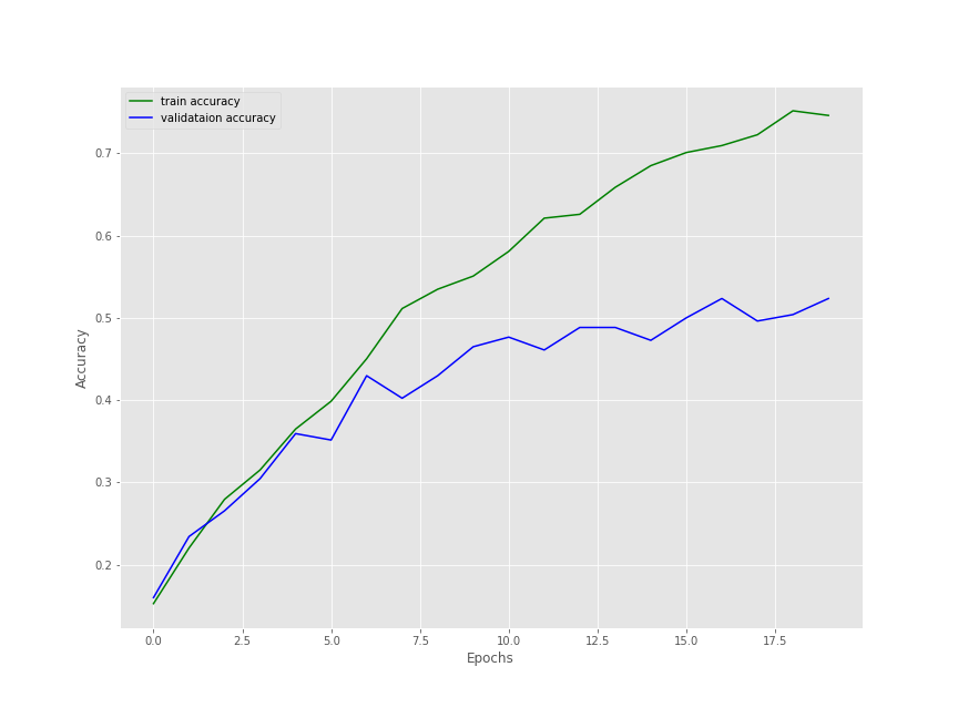
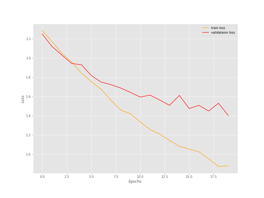
It is a bit difficult to say how well the training and validation would have gone if trained any further. But most probably, the results would have improved. You should surely try training for longer and see if there are any improvements in the results. If so, then surely let others know about your findings in the comment section.
A Few Takeaways
- When training on custom image data, we need to take care of the directory structure of the input data. If arranged properly, then the TensorFlow
ImageDataGeneratorwill take care of most of the work. - Using a complex image data requires a fairly complex model as well. A simple model might give good results during the training part, but the validation results might not be that good.
Summary and Conclusion
In this tutorial, you learned how to carry our image classification using TensorFlow in custom data. We learned to use the ImageDataGenerator class to prepare our image data for training. Then we built a simple neural network model for training on the monkey species image data. We also saw how a simple model might not give that good results while training. Most probably, we need to create a better model for this or try training for more epochs to get better results. You should surely give training on your own dataset a try and let others know about your results in the comment section. Mostly, our aim was to learn how to train a neural network in TensorFlow on a custom image dataset. I hope that you learned something new in this tutorial.
If you have any doubts, thoughts, or suggestions, then please leave them in the comment section. I will surely address them.
You can contact me using the Contact section. You can also find me on LinkedIn, and X.

Hello, I’m really interested on follow this tutorial, but the link to download the initial code isn’t working at the moment, could you please fix it, thanks!
Hello Rogelio. Sorry to hear that you are facing issues. Can you please check again? After you enter the email and press the button, it should lead you to a Google Drive download page.
If you still face issues, please email me at [email protected]