
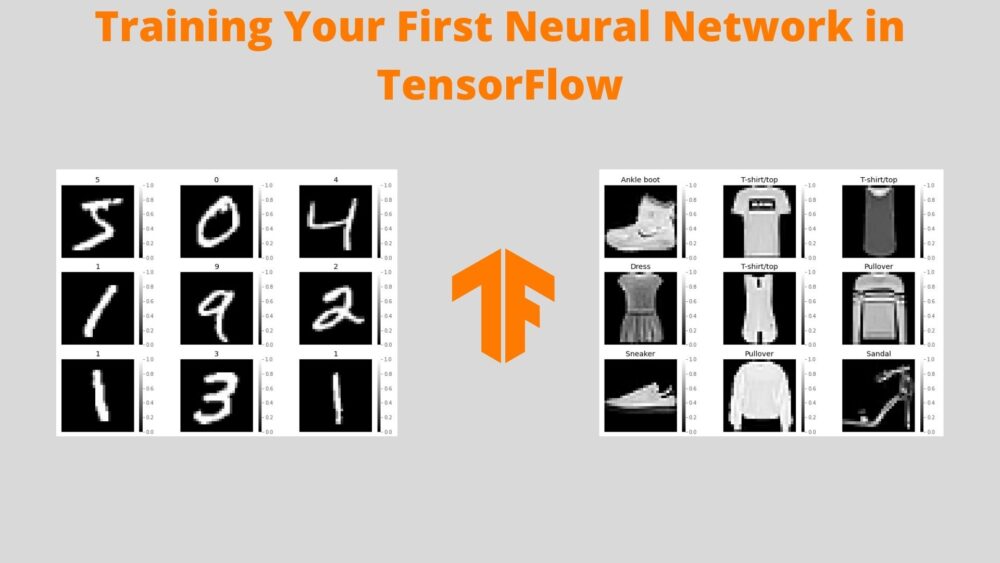
In this tutorial, you will learn how to train your first neural network in TensorFlow.
This post is the fourth in the series, Getting Started with TensorFlow.
- Introduction to Tensors in TensorFlow.
- Basics of TensorFlow GradientTape.
- Linear Regression using TensorFlow GradientTape.
- Training Your First Neural Network in TensorFlow.
If you are completely new to TensorFlow or just starting with deep learning, then going through the previous posts in the series will surely help you.
If you are somewhat familiar with TensorFlow by now, then going through this post will teach you how to build and train your first neural network model using TensorFlow.
We will cover the following topics in this tutorial.
- A Brief about the datasets that we will use.
- The Digit MNIST dataset.
- The Fashion MNIST dataset.
- Training a neural network in TensorFlow on the Digit MNIST dataset.
- Training a neural network in TensorFlow on the Fashion MNIST dataset.
For simplicity, we will build Dense neural networks in TensorFlow using Linear layers only. But in future posts of the series, we will cover convolutional neural networks as well on many interesting datasets. Also, going through this tutorial should give you a good sense of the general steps that we need to take for training a neural network using TensorFlow.
A Brief About the Datasets
We will use the Digit MNIST and Fashion MNIST datasets in this tutorial for training our neural networks. These are two very famous datasets for testing out new deep learning algorithms and models to know whether the model is working correctly or not. One more reason for choosing these datasets is that we can directly load these using TensorFlow functions. This greatly reduces the effort to download the data separately, preprocess them, and arrange them properly for training.
Although, the Digit MNIST dataset is getting quite old now and is mostly being replaced by the Fashion MNIST dataset. Still, it is a good starting point from a learning perspective.
The Digit MNIST Images
The Digit MNIST Images or more commonly known as the MNIST handwritten digits dataset. It contains 70000 images of handwritten digits.
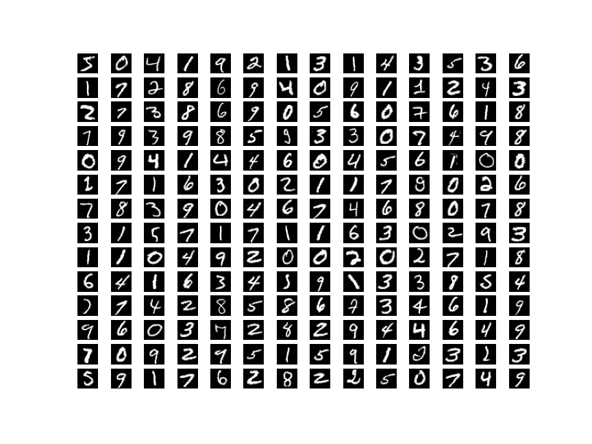
It contains handwritten digits from 0 to 9, so 10 classes in total. The data has already been preprocessed by resizing all images to a fixed size, that is 28×28. All images are grayscale which means they have only one color channel.
Out of these 70000 images, 60000 are training examples, and 10000 are test examples. This has become a very easy example to tackle nowadays with many advancements in computer vision and deep learning. But we can surely use this for learning new things in deep learning.
The Fashion MNIST Images
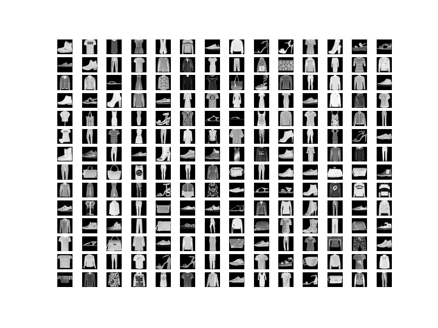
The Fashion MNIST dataset by Zalando is very similar to the Digit MNIST dataset. But instead of handwritten digits, it contains images of fashion items.
The following table shows all the fashion items present in the dataset.
| Label | Description |
|---|---|
| 0 | T-shirt/top |
| 1 | Trouser |
| 2 | Pullover |
| 3 | Dress |
| 4 | Coat |
| 5 | Sandal |
| 6 | Shirt |
| 7 | Sneaker |
| 8 | Bag |
| 9 | Ankle boot |
We can see that just like the Digit MNIST images, we have 10 classes in this dataset as well. All the images are in the grayscale format (single color channel) having 28×28 dimensions. There are 60000 training examples and 10000 test examples.
We will stop the discussion of the datasets here. If you want to learn a bit more about the datasets, then consider visiting the official websites.
Now, let’s start with the coding part of the tutorial.
The Directory Structure
Take a look at the directory structure that we will follow for this tutorial.
├── fashion_mnist.ipynb
├── mnist.ipynb
We have two Jupyter notebooks. One for the Digit MNIST dataset (mnist.ipynb) and one for the Fashion MNIST dataset (fashion_mnist.ipynb)
If you intend to code along while following the tutorial, I recommend using Jupyter notebooks. This will help you execute the code blocks sequentially and visualize the outputs right away. This is great for learning when starting with deep learning.
Training Your First Neural Network in TensorFlow
We will divide the remaining part of the tutorial into two sections. One for training our neural network on the Digit MNIST dataset and one for the training on the Fashion MNIST dataset.
Let’s start with the Digit MNIST part.
Training a Neural Network in TensorFlow on the Digit MNIST Dataset
The Digit MNIST training code will go into the mnist.ipynb Jupyter Notebook.
First, let’s import all the libraries and modules that we will need along the way.
import tensorflow as tf
import numpy as np
import matplotlib.pyplot as plt
import matplotlib
import numpy as np

from sklearn.metrics import classification_report

matplotlib.style.use('ggplot')
Along with all the standard imports, we are also importing the classification_report function from sklearn.metrics. We will use this to measure all the metrics on the test set after we have trained our model. These metrics are precision, recall, f1-score, support, and accuracy.
Import the Digit MNIST Dataset
We can load the Digit MNIST dataset directly using the tf.keras.datasets module.
mnist = tf.keras.datasets.mnist
(x_train, y_train), (x_test, y_test) = mnist.load_data()
print(f"Number of training images: {len(x_train)}")
print(f"Number of test images: {len(x_test)}")
We are loading the mnist dataset. This gets loaded in NumPy format. To get the full list of datasets, please visit this link.
x_trainholds all the training image pixel values andy_trainthe corresponding labels which range from 0 to 9.- Similarly,
x_testandy_testhold the test image pixel values and the labels.
We are printing the number of examples in each set just for a sanity check.
Number of training images: 60000
Number of test images: 10000
Visualize and Preprocess the Data
Let’s visualize the first image from the training set.
plt.imshow(x_train[0])
plt.colorbar()
plt.savefig('digit-mnist-single-digit.jpg')
plt.show()
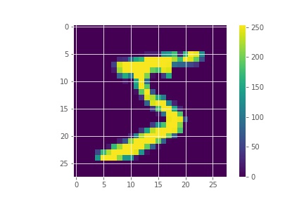
So, we get the digit 5. Notice one thing from the color bar. The current pixel values range between 0 and 255. This is a very varied range. To ensure that our neural network performs well, we will scale our values between 0 and 1 so that they have a similar scale. We will divide both the training set and the test set by 255.
x_train = x_train / 255.0
x_test = x_test / 255.0
Now, let’s visualize a few digits again with the corresponding labels and colorbar.
plt.figure(figsize=(12, 9))
for i in range(9):
    plt.subplot(3, 3, i+1)
    plt.axis('off')
    plt.imshow(x_train[i], cmap='gray')
    plt.colorbar()
    plt.title(y_train[i])
plt.savefig('digit-mnist-images-with-labels.jpg')
plt.show()
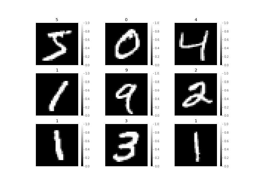
You can see all the labels on top of each digit in the above figure. This time we are showing the images in grayscale format. Take a look at the colorbar again. All the images have pixel values between 0 and 1. This indicates all the pixel values have been properly scaled.
Build and Train the Neural Network Model
In this section we will:
- First, stack the neural network layers. Our model will compose of
Denselayers only. - Second, we will compile the model.
- Finally, we will train the model for 10 epochs.
Stack the Neural Network Layers
The following code block contains the neural network architecture that we will use for training.
model = tf.keras.Sequential([
    tf.keras.layers.Flatten(input_shape=(28, 28)),
    tf.keras.layers.Dense(128, activation='relu'),
    tf.keras.layers.Dense(10)
])

print(model.summary())
We are creating a Sequential model.
- First, we are flattening the input image shape to 28×28=784 shape. This is because we are feeding our images to a
Denselayer. - Our first layer is a
Denselayer with 128 units. This is the only hidden layer we have. - The very next layer is also a
Denselayer and it acts as the output layer with 10 units as there are 10 classes in the Digit MNIST dataset.
Printing the model summary will give the following output.
Model: "sequential_2"
_________________________________________________________________
Layer (type)                 Output Shape              Param #
=================================================================
flatten (Flatten)            (None, 784)               0
_________________________________________________________________
dense_4 (Dense)              (None, 128)               100480
_________________________________________________________________
dense_5 (Dense)              (None, 10)                1290
=================================================================
Total params: 101,770
Trainable params: 101,770
Non-trainable params: 0
_________________________________________________________________
None
There are only 101,770 learnable parameters in the model. And do note that the Flatten layer does not have any learnable parameters. It just flattens the input.
Compile the Model
In TensorFlow, we need to compile the model first before we can train it. We need to provide the optimizer, the loss function, and the metric while compiling the model.
model.compile(
    optimizer='adam',
    loss=tf.keras.losses.SparseCategoricalCrossentropy(from_logits=True),
    metrics=['accuracy']
)
We are using the Adam optimizer, Sparse Categorical Cross Entropy as the loss function, and the metric is accuracy.
Train the Model
Now, we are all set to train the model. We just need to call the fit() function for that while providing the train images, train labels, and the number of epochs as arguments.
history = model.fit(x_train, y_train, epochs=10)
The following block shows the training step outputs.
Epoch 1/10
1875/1875 [==============================] - 2s 988us/step - loss: 0.2645 - accuracy: 0.9244
Epoch 2/10
1875/1875 [==============================] - 2s 938us/step - loss: 0.1154 - accuracy: 0.9660
Epoch 3/10
1875/1875 [==============================] - 2s 959us/step - loss: 0.0788 - accuracy: 0.9762
Epoch 4/10
1875/1875 [==============================] - 2s 894us/step - loss: 0.0585 - accuracy: 0.9822
Epoch 5/10
1875/1875 [==============================] - 2s 898us/step - loss: 0.0454 - accuracy: 0.9855
Epoch 6/10
1875/1875 [==============================] - 2s 943us/step - loss: 0.0355 - accuracy: 0.9886
Epoch 7/10
1875/1875 [==============================] - 2s 916us/step - loss: 0.0283 - accuracy: 0.99150
Epoch 8/10
1875/1875 [==============================] - 2s 911us/step - loss: 0.0227 - accuracy: 0.9928
Epoch 9/10
1875/1875 [==============================] - 2s 984us/step - loss: 0.0202 - accuracy: 0.9936
Epoch 10/10
1875/1875 [==============================] - 2s 904us/step - loss: 0.0149 - accuracy: 0.9955
By the end of the training, we are getting an accuracy of 99.55% and a loss of 0.0149. This looks pretty good for such a simple model and for just 10 training epochs.
Plot the Accuracy and Loss Line Graphs
Remember while training we executed the code as history = model.fit(). history is a dictionary that contains two keys, loss and accuracy. These two keys hold the loss and accuracy values for each of the 10 epochs respectively. We can very easily extract these values and plot the accuracy and loss graphs.
train_loss = history.history['loss']
train_acc = history.history['accuracy']

# accuracy plots
plt.figure(figsize=(10, 7))
plt.plot(
    train_acc, color='green', linestyle='-',
    label='train accuracy'
)
plt.xlabel('Epochs')
plt.ylabel('Accuracy')
plt.legend()
plt.savefig('digit-mnist-accuracy.jpg')
plt.show()
# loss plots
plt.figure(figsize=(10, 7))
plt.plot(
    train_loss, color='orange', linestyle='-',
    label='train loss'
)
plt.xlabel('Epochs')
plt.ylabel('Loss')
plt.legend()
plt.savefig('digit-mnist-loss.jpg')
plt.show()
Let’s take a look at the graphs.
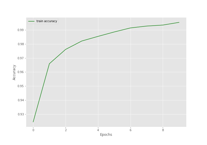
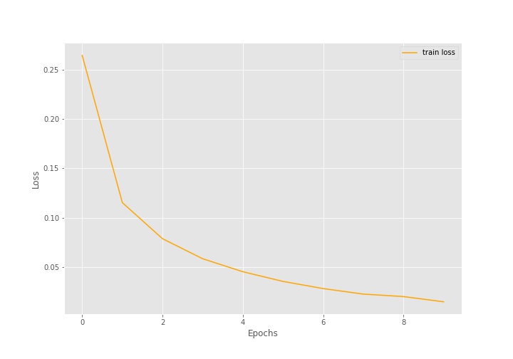
The accuracy line is increasing till the end of training and the loss line is decreasing. This is in exact accordance with what we saw during training.
Evaluation Accuracy and Loss on the Test Set
We also have a test set that we have not used till now. By now, we have a trained model. Let’s use this model to evaluate on the test set.
test_loss, test_acc = model.evaluate(x_test, y_test, verbose=1)
print(f"Test accuracy: {test_acc*100:.3f}")
print(f"Test loss: {test_loss:.3f}")
The evaluate() function accepts the test images and corresponding labels as the arguments. We are also passing verbose=1 so that it will show a progress bar.
The following is the output.
Test accuracy: 97.690
Test loss: 0.084
With just 10 epochs of training and such a simple model, we are getting 97.69% accuracy on the test set and a loss of 0.084. Will training for even more help improve the numbers? Do try that on your own and submit your findings in the comment section.
Generate the Classification Report
We can use Scikit-Learn’s classification_report() function to get a class-wise report of metrics on the test set. The following code shows how to do so.
y_pred = model.predict_classes(x_test)
cls_report = classification_report(y_test, y_pred)

for i in range(10):
    print(f"Class {i}: Digit {i}")
print(cls_report)
We are using the predict_classes() function to get all the predictions on the test set which are stored in y_pred. y_pred is a NumPy array that contains the resulting classes for the 10000 test images.
Then we are using the classification_report() function while passing the true test labels y_test, and the predicted class labels y_pred as the arguments. This provides us with the classification report. For better understanding, we are running a for loop to print which digit belongs to which class so that everything will be clear when taking a look at the classification report. The following is the output.
Class 0: Digit 0
Class 1: Digit 1
Class 2: Digit 2
Class 3: Digit 3
Class 4: Digit 4
Class 5: Digit 5
Class 6: Digit 6
Class 7: Digit 7
Class 8: Digit 8
Class 9: Digit 9
              precision    recall  f1-score   support

           0       0.99      0.99      0.99       980
           1       0.99      0.99      0.99      1135
           2       0.97      0.99      0.98      1032
           3       0.96      0.99      0.97      1010
           4       0.99      0.97      0.98       982
           5       0.98      0.97      0.97       892
           6       0.98      0.97      0.98       958
           7       0.97      0.98      0.98      1028
           8       0.98      0.96      0.97       974
           9       0.98      0.97      0.97      1009

    accuracy                           0.98     10000
   macro avg       0.98      0.98      0.98     10000
weighted avg       0.98      0.98      0.98     10000
We have the precision, recall, f1-score, and support for each class. Then we also have an accuracy of 98% which matches with the accuracy we got using the evaluate() function. The classification report can provide a lot of insights when dealing with complex datasets and to know if the model is learning the features of one class better or worse than others.
This brings us to the end of training our first neural network using TensorFlow on the Digit MNIST dataset.
As discussed, we will train a neural network on the Fashion MNIST dataset as well. Let’s get on to that without any further delay.
Training a Neural Network in TensorFlow on the Fashion MNIST Dataset
From this section onward, we will write the code to train a neural network on the Fashion MNIST dataset. Note that we will keep all of the code the same except the dataset. This section is mostly for learning purposes as the Fashion MNIST data is slightly more complex to tackle when compared to the Digit MNIST dataset. We will see how the same model compares to when trying to learn the features of the Fashion MNIST images.
We will write this code in the fashion_mnist.ipynb Jupyter notebook.
Import the Required Modules and Libraries
Let’s import everything first.
import tensorflow as tf
import numpy as np
import matplotlib.pyplot as plt
import matplotlib
import numpy as np

from sklearn.metrics import classification_report

matplotlib.style.use('ggplot')
Import the Fashion MNIST Dataset
Let’s import and load the dataset.
fashion_mnist = tf.keras.datasets.fashion_mnist
(x_train, y_train), (x_test, y_test) = fashion_mnist.load_data()
print(f"Number of training images: {len(x_train)}")
print(f"Number of test images: {len(x_test)}")
Number of training images: 60000
Number of test images: 10000
Just like the Digit MNIST dataset, Fashion MNIST has 60000 training and 10000 test examples.
But what about the labels? We know that the images belong to clothing materials. So, how are the labels represented in the data?
print(y_train)
[9 0 0 ... 3 0 5]
The labels are just numbers. 0 corresponds to T-shirt/top class, 1 corresponds to Trouser class and so on. While visualizing the images, it will be a lot more intuitive if we can know the actual name of the clothing material. For that, let’s create a list containing all the clothing item names which we can easily map using the class numbers later on.
class_names = ['T-shirt/top', 'Trouser', 'Pullover', 'Dress', 'Coat',
               'Sandal', 'Shirt', 'Sneaker', 'Bag', 'Ankle boot']
The class_names list contains the names of all the clothing materials.
Visualize and Preprocess the Data
Let’s visualize one image without scaling the pixel values.
plt.imshow(x_train[0])
plt.colorbar()
plt.savefig('fashion-mnist-apparel.jpg')
plt.show()
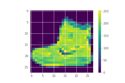
The above image shows an ankle boot and the pixel values are between 0 and 255.
Let’s scale the values and visualize a few images with the labels.
x_train = x_train / 255.0
x_test = x_test / 255.0
plt.figure(figsize=(12, 9))
for i in range(9):
    plt.subplot(3, 3, i+1)
    plt.axis('off')
    plt.imshow(x_train[i], cmap='gray')
    plt.colorbar()
    plt.title(class_names[y_train[i]])
plt.savefig('fashion-mnist-images-with-labels.jpg')
plt.show()
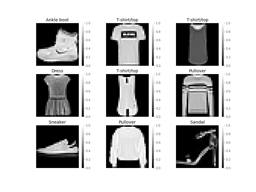
Now, the pixel values are between 0 and 1 and we can see the true labels on top of each fashion item as well.
Build and Train the Neural Network Model
Let’s start the process of building, compiling, and training the neural network model.
Stack the Layers
We will use the same model as we did in the case of Digit MNIST training. Now, we know that the Fashion MNIST images are a bit more complex to learn than the Digit MNIST dataset. So, the same model might not perform just as well. And we will get to know how much the complexity of data matters in choosing how complex our model should be.
model = tf.keras.Sequential([
    tf.keras.layers.Flatten(input_shape=(28, 28)),
    tf.keras.layers.Dense(128, activation='relu'),
    tf.keras.layers.Dense(10)
])

print(model.summary())
Model: "sequential"
_________________________________________________________________
Layer (type)                 Output Shape              Param #
=================================================================
flatten (Flatten)            (None, 784)               0
_________________________________________________________________
dense (Dense)                (None, 128)               100480
_________________________________________________________________
dense_1 (Dense)              (None, 10)                1290
=================================================================
Total params: 101,770
Trainable params: 101,770
Non-trainable params: 0
_________________________________________________________________
None
Compile the Model
We use the Adam optimizer, Sparse Categorical Cross-Entropy as loss, and accuracy as the metric.
model.compile(
    optimizer='adam',
    loss=tf.keras.losses.SparseCategoricalCrossentropy(from_logits=True),
    metrics=['accuracy']
)
Train the Model
Now, training the model for 10 epochs.
history = model.fit(x_train, y_train, epochs=10)
Epoch 1/10
1875/1875 [==============================] - 2s 883us/step - loss: 0.4947 - accuracy: 0.8255
Epoch 2/10
1875/1875 [==============================] - 2s 896us/step - loss: 0.3744 - accuracy: 0.8659
Epoch 3/10
1875/1875 [==============================] - 2s 876us/step - loss: 0.3367 - accuracy: 0.8787
Epoch 4/10
1875/1875 [==============================] - 2s 947us/step - loss: 0.3141 - accuracy: 0.8847
Epoch 5/10
1875/1875 [==============================] - 2s 1ms/step - loss: 0.2949 - accuracy: 0.8911
Epoch 6/10
1875/1875 [==============================] - 2s 1ms/step - loss: 0.2810 - accuracy: 0.8946
Epoch 7/10
1875/1875 [==============================] - 2s 919us/step - loss: 0.2692 - accuracy: 0.9005
Epoch 8/10
1875/1875 [==============================] - 2s 885us/step - loss: 0.2563 - accuracy: 0.9039
Epoch 9/10
1875/1875 [==============================] - 2s 900us/step - loss: 0.2495 - accuracy: 0.9061
Epoch 10/10
1875/1875 [==============================] - 2s 898us/step - loss: 0.2383 - accuracy: 0.9105
After training for 10 epochs, the accuracy is 91.05% which is obviously lower than what we got while training the Digit MNIST dataset. And the loss of 0.2383 is also higher than the previous case.
Plot the Accuracy and Loss Line Graphs
Let’s plot the accuracy and loss graphs now.
train_loss = history.history['loss']
train_acc = history.history['accuracy']

# accuracy plot
plt.figure(figsize=(10, 7))
plt.plot(
    train_acc, color='green', linestyle='-',
    label='train accuracy'
)
plt.xlabel('Epochs')
plt.ylabel('Accuracy')
plt.legend()
plt.savefig('fashion-mnist-accuracy.jpg')
plt.show()
# loss plot
plt.figure(figsize=(10, 7))
plt.plot(
    train_loss, color='orange', linestyle='-',
    label='train loss'
)
plt.xlabel('Epochs')
plt.ylabel('Loss')
plt.legend()
plt.savefig('fashion-mnist-loss.jpg')
plt.show()
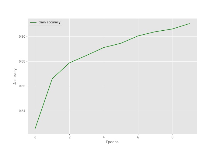
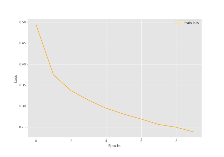
Looking at the graphs, we can get a sense that training for more epochs will have increased the accuracy and decreased the loss as well.
Evaluation Accuracy and Loss on the Test Set
The following code evaluates the neural network model on the test set and prints the results.
test_loss, test_acc = model.evaluate(x_test, y_test, verbose=1)
print(f"Test accuracy: {test_acc*100:.3f}")
print(f"Test loss: {test_loss:.3f}")
Test accuracy: 88.360
Test loss: 0.340
The test accuracy is 88.36% and the test loss is 0.340. We had got better results in the case of Digit MNIST test set evaluation while using the same model.
Generate the Classification Report
Finally, we will generate the classification report for the true labels and predicted labels.
y_pred = model.predict_classes(x_test)
cls_report = classification_report(y_test, y_pred)

for i in range(len(class_names)):
    print(f"Class {i}: {class_names[i]}")
print(cls_report)
Class 0: T-shirt/top
Class 1: Trouser
Class 2: Pullover
Class 3: Dress
Class 4: Coat
Class 5: Sandal
Class 6: Shirt
Class 7: Sneaker
Class 8: Bag
Class 9: Ankle boot
              precision    recall  f1-score   support

           0       0.77      0.91      0.83      1000
           1       0.96      0.98      0.97      1000
           2       0.75      0.85      0.80      1000
           3       0.92      0.85      0.88      1000
           4       0.81      0.79      0.80      1000
           5       0.97      0.96      0.97      1000
           6       0.79      0.58      0.67      1000
           7       0.95      0.96      0.96      1000
           8       0.98      0.97      0.97      1000
           9       0.95      0.97      0.96      1000

    accuracy                           0.88     10000
   macro avg       0.89      0.88      0.88     10000
weighted avg       0.89      0.88      0.88     10000
While the precision for all the classes was above 90% in case of Digit MNIST, for the Fashion MNIST images, we have precision as low as 75% for the Pullover clothe images.
This shows how important it is to take into account the model complexity as our dataset complexity increases.
A Few Takeaways and Further Experiments
- We saw that the same simple model might not perform very well on a complex dataset.
- If the dataset complexity increases, then training for more number of epochs might also help.
- You can try adding a few more hidden layers to the current model and train again on the Fashion MNIST dataset. Try training for more epochs as well and let others know about your results in the comment section. This is will be good learning experience for all.
Summary and Conclusion
In this tutorial, we built and trained our first neural network using TensorFlow on the Digit MNIST and Fashion MNIST dataset. The model consisted of Dense layers only and we will see how to build and train convolutional neural networks as well in future posts of the series. I hope that you learned something new from this tutorial.
If you have any doubts, thoughts, or suggestions, then please leave them in the comment section. I will surely address them.
You can contact me using the Contact section. You can also find me on LinkedIn, and X.

hello, we just test your tutorial and it works perfectly, thanks.
we are an open source informatis school in africa, cameroon limbe and we want to introduce ai, machine learning in our school, but…we have nobody who really master this topic. we have done some exercise with opencv python, but the how to build datasets, tensor flow, teras is new. so what do you propose? exist good tutorials, any help will help us, thanks
association linux friends limbe
Hello Michel, I am happy that you find the tutorials here helpful. Please send an email at [email protected] and let’s see how we can proceed further and how we can take this proposition further. Email is much better for extended information sharing. I will be very happy to help.
Very good tutorial. I really appreciate a lot.
I have some questions here. Could you please help to write in developing the code for our own taken Image datasets in CNN. That is I wish to replace here …
(x_train, y_train), (x_test, y_test) = fashion_mnist.load_data()
in this “fashion_mnist.load_data()” I wish to keep/load my own dataset. If possible please assist me on this. Thanks in advance
Hello Ramkumar. In the following blog post, I show how to use TensorFlow on a custom dataset. Maybe this will help you.
https://debuggercafe.com/transfer-learning-using-tensorflow/