Plant Disease Recognition using Deep Learning and PyTorch

In this post, we will train a deep learning model for plant disease recognition.

Using deep learning and machine learning has helped to solve many agricultural issues. Deep learning based computer vision systems have been especially helpful. Such deep learning systems/models can easily recognize different diseases in plants when we train them on the right dataset. For example, we can train a deep learning model to recognize different types of diseases in rice leaves.

Most of the time, obtaining large and well-defined datasets to solve such problems becomes an issue. Because for deep learning models to recognize diseases in plants, they will need to train on huge amounts of data. But that does not mean we cannot train a simple deep learning model to check whether such models can work or not.

In fact, in this blog post, we will use around 1300 images for training a deep learning model. For plant disease recognition, this may not seem much. But as we will see later on, this is a good starting point, which gives us a deep learning model that works fairly well.

In this blog post, we will start simple, and gradually expand this to broader and more difficult problems for agricultural applications. We will solve more such practical applications in future posts.

Points to Cover in the Post

• We will start with the discussion of the plant disease recognition dataset that we will use.
• For the training and coding section, we will discuss:
  • The deep learning model that we use for plant disease recognition.
  • The augmentations to apply to the images and how they affect the results.
• After training, completes, we will also test our model and visualize the class activation maps.

Let’s move ahead.

The Plant Disease Recognition Dataset

We will use the plant disease recognition dataset from Kaggle to train a deep learning model in this post.

The dataset contains images of leaves from different plants which may or may not be affected by a disease.

This dataset contains a total of 1530 images with three classes:

• Healthy: Leaves with no diseases.
• Powdery: These are the leaves that are affected by powdery mildew disease. It is a type of fungal disease that can affect plants based on the time of year. You can read more about the disease here.
• Rust: The rust disease can affect different plants. It is a type of fungal disease as well. You may read more about it here.

The following are some of the images from the dataset along with the different types of diseases they are classified into.

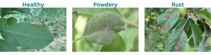
As you may see, it is pretty easy to identify the powdery and rust diseases even with the naked eye. Further on, we will get to know how well a deep learning based image classification model performs on the dataset.

The dataset has already been split into three sets:

• Train: The training set contains 1322 images.
• Validation: The validation set contains 60 images.
• Test: The test set contains 150 images.

The dataset is fairly balanced among the three classes. This is good for training a deep learning model.

Before moving further, you may download the dataset from here if you wish to run the training experiments on your local system.

Directory Structure

The following is the structure of all the directories and files that we use in this project.

.
├── input
│   ├── Test
│   │   └── Test
│   │       ├── Healthy
│   │       ├── Powdery
│   │       └── Rust
│   ├── Train
│   │   └── Train
│   │       ├── Healthy
│   │       ├── Powdery
│   │       └── Rust
│   └── Validation
│       └── Validation
│           ├── Healthy
│           ├── Powdery
│           └── Rust
├── notebooks
│   └── visualize_augmentations.ipynb
├── outputs
│   ├── cam_results [150 entries exceeds filelimit, not opening dir]
│   ├── test_results [150 entries exceeds filelimit, not opening dir]
│   ├── accuracy.png
│   ├── loss.png
│   └── model.pth
└── src
    ├── cam.py
    ├── datasets.py
    ├── model.py
    ├── test.py
    ├── train.py
    └── utils.py

• In the above directory structure, we have the extracted dataset in the input directory. It contains subdirectories for the three splits. The images of each class are present in their respective folders.
• The outputs directory contains the results that we obtain from training and testing the deep learning model.
• The notebooks directory contains a single Jupyter Notebook for visualizing augmented images.
• Finally, the src directory contains the Python code files. We will explore a few of the important contents of these files in further sections of this post.

When downloading the zip file for this post, you will get access to all the code files and the trained model as well. If you wish to train the model on your own, then you may download the dataset and arrange it as per the above structure in the input directory.

PyTorch Version

The code in this post uses PyTorch version 1.12.1 along with Torchvision 0.13.0. Later versions (if available) will also work.

Plant Disease Recognition using Deep Learning and PyTorch

In this section, we will discuss some of the important practical aspects of the training pipeline, and the dataset preparation.

We will not discuss the Python files in detail here. Just the important sections. All the code files are still available through the downloadable zip file.

The Deep Learning Model (ResNet34)

For training, we will use a pretrained ResNet34 network and fine-tune it on the plant disease dataset.

Download Code

We use the model from Torchvision which has already been pretrained on the ImageNet dataset. Preparing the ResNet34 model is pretty easy and takes a few lines of code only. The following block contains the entire code which goes into the model.py file.

import torch.nn as nn

from torchvision import models
from torchvision.models import ResNet34_Weights

def build_model(pretrained=True, fine_tune=True, num_classes=10):
    if pretrained:
        print('[INFO]: Loading pre-trained weights')
        model = models.resnet34(weights=ResNet34_Weights.DEFAULT)
    else:
        print('[INFO]: Not loading pre-trained weights')
        model = models.resnet34(weights=None)
        
    if fine_tune:
        print('[INFO]: Fine-tuning all layers...')
        for params in model.parameters():
            params.requires_grad = True
    elif not fine_tune:
        print('[INFO]: Freezing hidden layers...')
        for params in model.parameters():
            params.requires_grad = False

    # Change the final classification head.
    model.fc = nn.Linear(in_features=512, out_features=num_classes)
    return model

As you can see, we need to change the final fully connected layer. The number of classes has been changed from 1000 (for ImageNet) to 3 (for the plant disease recognition dataset).

Experiments with other models were also done, but they did not work very well. The ResNet family of models worked pretty well and most probably ResNet50 will work even better.

Dataset Preparation for Training

Coming to the dataset preparation part. All the code is available in the datasets.py file.

Here, we will discuss the hyperparameters for dataset preparation and the augmentations used.

IMAGE_SIZE = 224 # Image size of resize when applying transforms.
BATCH_SIZE = 32

We choose an image size of 224×224 resolution. Higher resolutions will also work well but will require more GPU memory and longer training time. From the experiments, lower resolutions did not work very well.

For the batch size, 32 gave pretty good results, as we will see later on. If you train on your local system and run out of GPU memory (OOM), try reducing the batch size. But reducing the batch size may require longer training to reach the same accuracy as with a batch size of 32. This is something to experiment with.

We also use a few transforms and augmentations. The augmentations help to reduce overfitting and also allow us to train for longer. The following snippets show the transforms/augmentations for the training and validation set.

# Training transforms
def get_train_transform(image_size):
    train_transform = transforms.Compose([
        transforms.Resize((image_size, image_size)),
        transforms.RandomHorizontalFlip(p=0.5),
        transforms.RandomRotation(35),
        transforms.RandomAdjustSharpness(sharpness_factor=2, p=0.5),
        transforms.ToTensor(),
        transforms.Normalize(
            mean=[0.485, 0.456, 0.406],
            std=[0.229, 0.224, 0.225]
            )
    ])
    return train_transform

# Validation transforms
def get_valid_transform(image_size):
    valid_transform = transforms.Compose([
        transforms.Resize((image_size, image_size)),
        transforms.ToTensor(),
        transforms.Normalize(
            mean=[0.485, 0.456, 0.406],
            std=[0.229, 0.224, 0.225]
            )
    ])
    return valid_transform

For the training set, we choose three augmentations. They are horizontal flipping, random rotation, and random application of sharpness to the images.

For reference, this is what some of the augmented images from the training set look like.

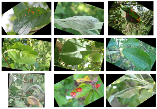
Other than that, for both, the training and the validation set, we will use the ImageNet normalization values. This is because we are fine-tuning a pretrained ResNet34 model.

The rest of the dataset preparation code contains creating the datasets and the data loaders.

Training the ResNet34 Model for Plant Disease Recognition

In this section, we will run the training script, that is train.py, and check out the results.

Before that, let’s see the hyperparameters and parameters that we use for training.

• We will be training for 20 epochs. You can change this by passing --epochs argument in the command line while executing train.py.
• The optimizer is SGD with momentum and the learning is 0.001. The learning rate can also be passed through the command line. Use the --learning-rate argument for this.
• As it is a multi-class problem, we are using the Cross-Entropy loss function.

To begin training, execute the following command within the src directory.

python train.py --epochs 20

The following are some of the truncated outputs from the terminal.

[INFO]: Number of training images: 1322
[INFO]: Number of validation images: 60
[INFO]: Classes: ['Healthy', 'Powdery', 'Rust']
Computation device: cuda
Learning rate: 0.001
Epochs to train for: 20

[INFO]: Loading pre-trained weights
[INFO]: Fine-tuning all layers...
21,286,211 total parameters.
21,286,211 training parameters.
[INFO]: Epoch 1 of 20
Training
100%|████████████████████████████████████████████████████████████████████| 42/42 [00:26<00:00,  1.57it/s]
Validation
100%|██████████████████████████████████████████████████████████████████████| 2/2 [00:02<00:00,  1.24s/it]
Training loss: 0.530, training acc: 77.912
Validation loss: 0.086, validation acc: 100.000
--------------------------------------------------
.
.
.
[INFO]: Epoch 20 of 20
Training
100%|████████████████████████████████████████████████████████████████████| 42/42 [00:25<00:00,  1.63it/s]
Validation
100%|██████████████████████████████████████████████████████████████████████| 2/2 [00:02<00:00,  1.19s/it]
Training loss: 0.003, training acc: 99.924
Validation loss: 0.001, validation acc: 100.000
--------------------------------------------------
TRAINING COMPLETE

As you may see, we are getting almost 100% training accuracy. The validation accuracy is already 100%. The training accuracy may be a bit lower because of the augmentations. Looks like training a few more epochs would give slightly better training results as well.

Let’s take a look at the accuracy and loss graphs.

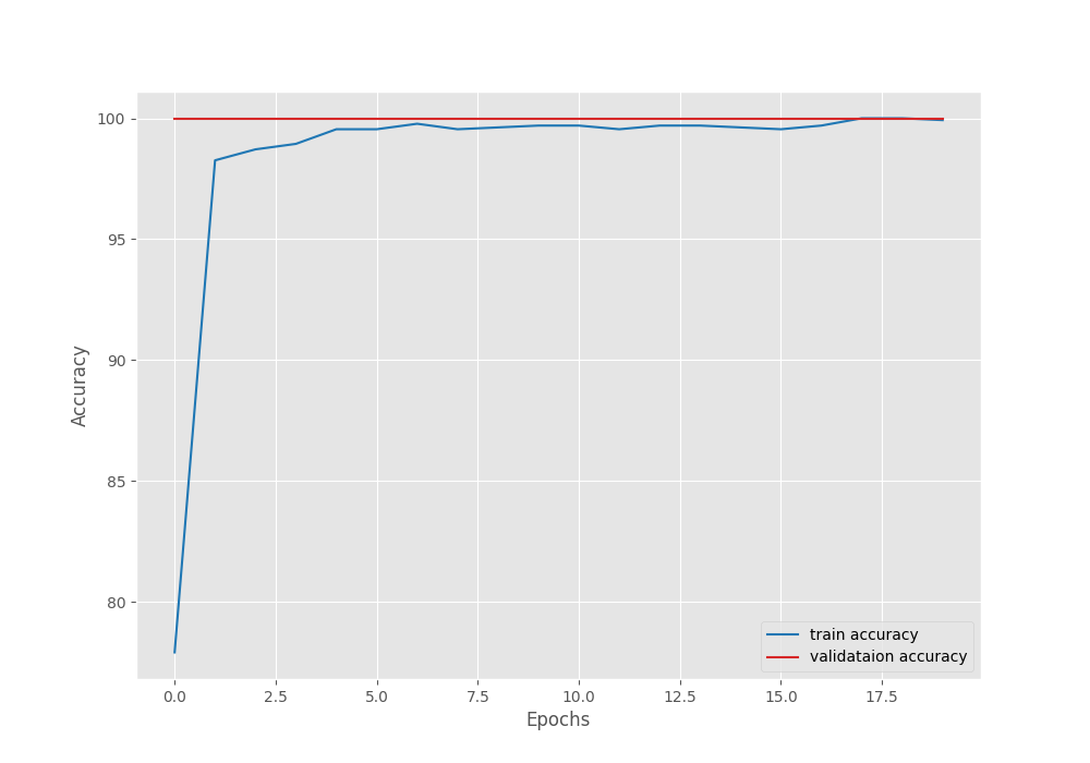
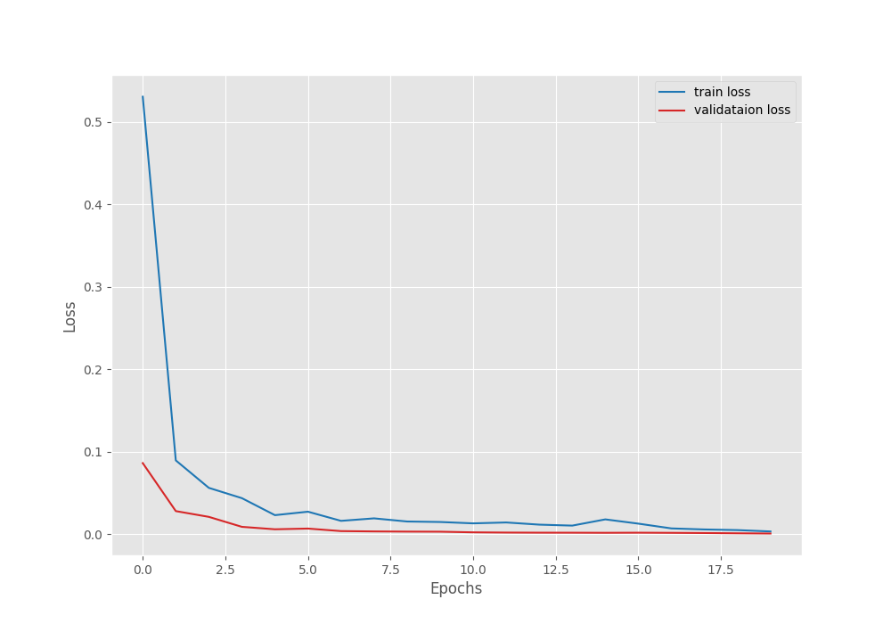
As we can see, the validation accuracy is already 100% from the very first epoch. This happens when using the momentum factor along with the SGD optimizer. Without the momentum factor, the convergence is slightly slower.

Testing the Trained Model for Plant Disease Recognition

We already have the trained model with us. This section will accomplish two things.

• Run the trained model on the test images using the test.py script.
• Visualize the class activation maps on the test image using the cam.py script.

To run the test script, execute the following command in the terminal.

python test.py 

The following are the results.

python test.py 
[INFO]: Not loading pre-trained weights
[INFO]: Freezing hidden layers...
Testing model
100%|██████████████████████████████████████████████████████████████████| 150/150 [00:04<00:00, 33.20it/s]
Test accuracy: 97.333%

With the currently trained model, we get more than 97% accuracy.

The following are some of the results are saved to the disk.

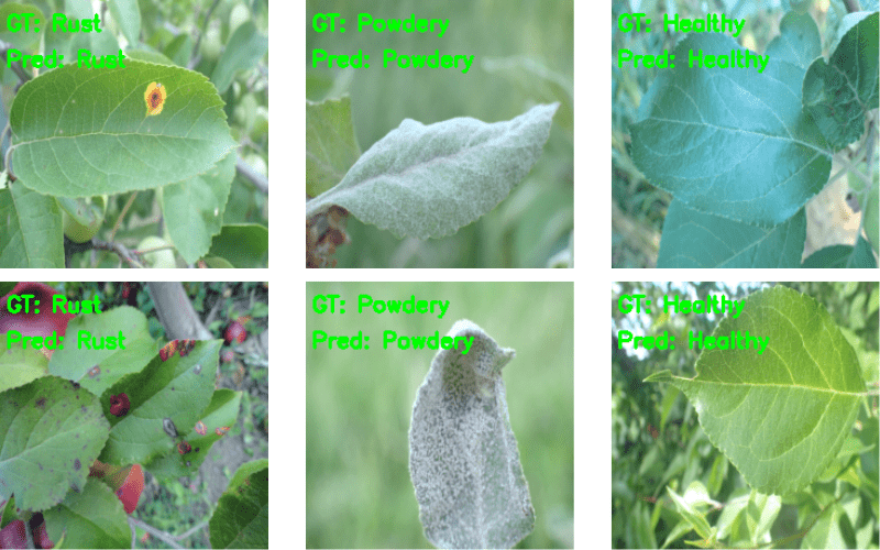
The above image shows some of the correct predictions made by the model.

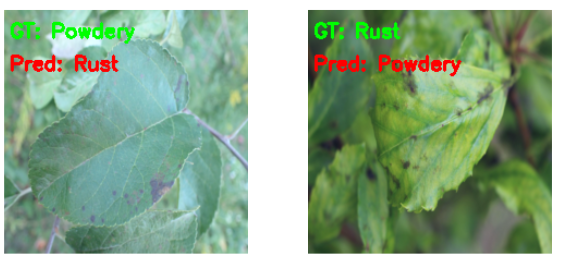
Figure 7 shows two wrong predictions made by the model.

For the image on the left, the ground truth is Powdery. But it looks more like a labeling error and it seems to be the Rust disease. For the image on the right, the model is predicting the disease as Powdery whereas it is actually Rust.

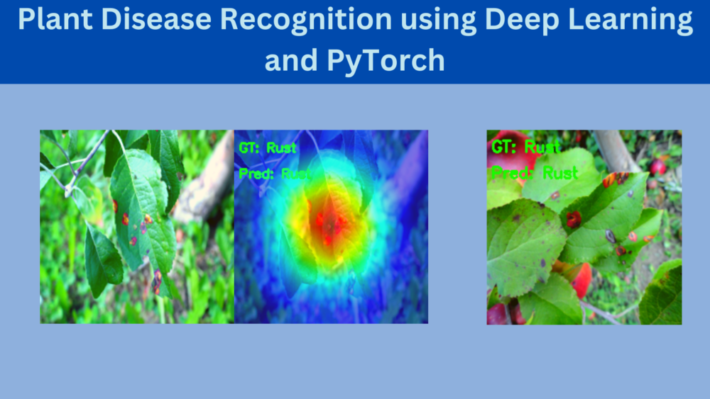
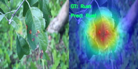
Now, to visualize the class activation maps, run the following command.

python cam.py

The above will carry out the testing of the model as well. But we are interested only in the class activation maps which are saved in the outputs/cam_results directory.

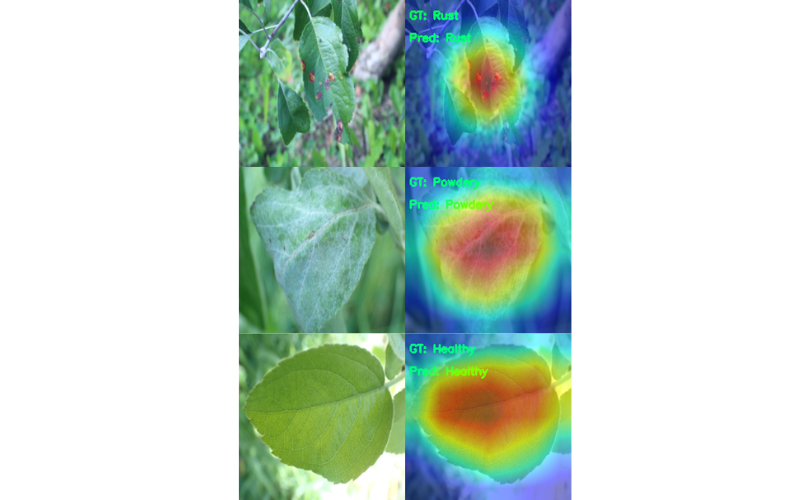
It is clearly visible that the model is specifically focusing on the diseased area of the leaf while making the predictions. It is very evident from the Rust disease where the model looks at the spots and makes the predictions.

Summary and Conclusion

In this blog post, we used deep learning to solve a real-world problem on a small scale. We trained a ResNet34 model for plant disease recognition. After training the model, we tested it on the test set and also visualized the class activation maps. This gave us better insights into what the model is looking at while making predictions. Hopefully, this post was helpful for you.

If you have any doubts, thoughts, or suggestions, please leave them in the comment section. They will surely be addressed.

You can contact me using the Contact section. You can also find me on LinkedIn, and Twitter.