

In this post, we will try to train a deep neural network model for recognizing rice leaf disease. Deep learning and computer vision are helping solve many real-world issues. And in this post, we will check whether deep learning can help with rice leaf disease recognition.
This will be a bit challenging as we will use a very small dataset for training and validation. Then try to use real-world unseen images from the internet for inference. Building and validating a good-performing model will be a bit difficult. Still, we will try our best.
We will cover the following topics in this post:
- We will start with an exploration of the rice leaf disease images dataset. This includes:
- Exploring the images.
- The number of classes.
- Then we will move on to discuss the directory structure of the project.
- Next, we will start the coding part for rice leaf disease recognition using deep learning.
- After training the model, we will move to the inference part. This will tell how well our model performs on unseen real-world data.
- Finally, we will discuss what will be some of the possible next steps if we want to extend this project further.
Now, let’s move on to the details of the post.
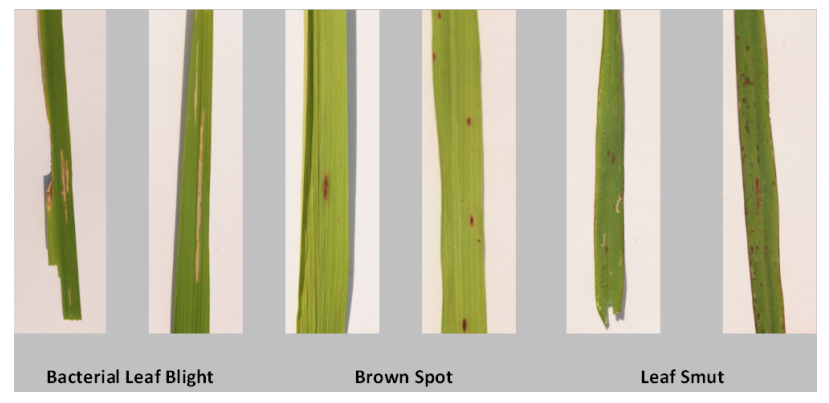
The Rice Leaf Disease Dataset
We will use the Rice Leaf Diseases Dataset from Kaggle in this post. This dataset contains 120 images of diseased rice leaves belonging to three different classes. The classes are:
- Leaf smut
- Brown spot
- Bacterial leaf blight
The following image gives a pretty good idea of each rice leaf disease.
We can see that the three diseases look different when they affect the rive leaves. Detecting such diseases manually may be possible, but is surely time-consuming. Probably, trying to automate this disease recognition process using machine learning is a good idea. This will lead to faster diagnosing of the disease and at many times to even faster treatment.
In this dataset, we don’t have many images. Only 40 images per class. That’s why it’s going to be pretty challenging to build a robust deep learning model that can recognize each disease with good accuracy. Moreover, we have to use a lot of augmentation techniques as well. We will get into all the technical details when writing the code.
The Directory Structure
Let’s take a look at the directory structure of the project.
├── input
│   ├── rice_leaf_diseases
│   │   ├── Bacterial leaf blight [40 entries exceeds filelimit, not opening dir]
│   │   ├── Brown spot [40 entries exceeds filelimit, not opening dir]
│   │   └── Leaf smut [40 entries exceeds filelimit, not opening dir]
│   └── test_data
│       ├── bacterial_leaf_blight.jpg
│       ├── brown_spot.png
│       └── leaf_smut.png
├── outputs
│   ├── accuracy.png
│   ├── bacterial_leaf_blight.png
│   ├── brown_spot.png
│   ├── leaf_smut.png
│   ├── loss.png
│   └── model.pth
├── src
│   ├── datasets.py
│   ├── inference.py
│   ├── model.py
│   ├── train.py
│   └── utils.py
- The
inputdirectory contains the dataset that is,rice_leaf_diseases. Inside it, there are three class directories each containing 40 images belonging to that class. It also contains atest_datadirectory which holds three images that we will use for inference after we train our model. - The
outputsdirectory will contain the trained model, the loss and accuracy plots, and even the inference image results. - Finally, the
srcdirectory contains the five Python files for which we need to write the code in this post.
If you download the zip file for this post, you will get all the files and folders in place. This will also contain the dataset and trained model. After extracting it, you can either train the model on your own or run the inference using the trained model.
The PyTorch Version
The code in this post has been developed using PyTorch version 1.10. It is better if you have the same or newer version as well. If you need to install/upgrade your PyTorch locally, you can head over here.
Rice Leaf Disease Recognition using Deep Learning
From here, we will start with the coding part of the post. Most of the things will be similar to any other image classification code using PyTorch. We will surely dive deep into the coding part which requires attention.
We will start with writing a few helper functions.
Helper Functions for Saving Graphs and Trained Model
We will write two helper functions. One for saving the graphs for accuracy and loss and the other one for saving the trained model.
The helper functions code will go into the utils.py file.
The first code block contains the import statements and also the function to save the trained model.
import torch
import matplotlib
import matplotlib.pyplot as plt

matplotlib.style.use('ggplot')

def save_model(epochs, model, optimizer, criterion):
    """
    Function to save the trained model to disk.
    """
    torch.save({
                'epoch': epochs,
                'model_state_dict': model.state_dict(),
                'optimizer_state_dict': optimizer.state_dict(),
                'loss': criterion,
                }, f"../outputs/model.pth")
Along with the model state dictionary, we also save the number of epochs trained for, the optimizer state dictionary, and also the loss function. All of this will help us resume training in the future if we are able to collect more data.
The next function is for saving the accuracy and loss graphs.
def save_plots(train_acc, valid_acc, train_loss, valid_loss):
    """
    Function to save the loss and accuracy plots to disk.
    """
    # Accuracy plots.
    plt.figure(figsize=(10, 7))
    plt.plot(
        train_acc, color='green', linestyle='-',
        label='train accuracy'
    )
    plt.plot(
        valid_acc, color='blue', linestyle='-',
        label='validataion accuracy'
    )
    plt.xlabel('Epochs')
    plt.ylabel('Accuracy')
    plt.legend()
    plt.savefig(f"../outputs/accuracy.png")

    # Loss plots.
    plt.figure(figsize=(10, 7))
    plt.plot(
        train_loss, color='orange', linestyle='-',
        label='train loss'
    )
    plt.plot(
        valid_loss, color='red', linestyle='-',
        label='validataion loss'
    )
    plt.xlabel('Epochs')
    plt.ylabel('Loss')
    plt.legend()
    plt.savefig(f"../outputs/loss.png")
The save_plots() function accepts the list containing the training & validation accuracy, and training & validation loss values. It saves the plots in the outputs directory.
The above two are the helper functions that we need.
Preparing the Dataset
The next step is to prepare the dataset. All the images are inside the rice_leaf_diseases directory without any training or validation split. We will do the splitting on our own.
The dataset preparation code will go into the datasets.py file.
Starting with the import statements and a few constants that we need along the way.
import torch

from torchvision import datasets, transforms
from torch.utils.data import DataLoader, Subset

# Required constants.
ROOT_DIR = '../input/rice_leaf_diseases'
VALID_SPLIT = 0.1
IMAGE_SIZE = 224 # Image size of resize when applying transforms.
BATCH_SIZE = 16
NUM_WORKERS = 4 # Number of parallel processes for data preparation.
We need the Subset class to divide the data into a train and validation set. Then we also define a few constants for the root data directory, the validation split ratio, the image size to resize to during transforms, the batch size, and the number of workers. We are using 10% of the data for validation and the rest for training. That would be around 12 validation images.
The Training and Validation Transforms
Next, we will define the training and validation transforms. First, let’s check out the code, then we will get into the details.
# Training transforms
def get_train_transform(IMAGE_SIZE):
    train_transform = transforms.Compose([
        transforms.Resize((IMAGE_SIZE, IMAGE_SIZE)),
        transforms.RandomHorizontalFlip(p=0.5),
        transforms.RandomVerticalFlip(p=0.5),
        transforms.GaussianBlur(kernel_size=(5, 9), sigma=(0.1, 5)),
        transforms.RandomAdjustSharpness(sharpness_factor=2, p=0.5),
        transforms.RandomAutocontrast(p=0.5),
        transforms.RandomGrayscale(p=0.5),
        transforms.RandomRotation(45),
        transforms.ToTensor(),
        transforms.Normalize(
            mean=[0.485, 0.456, 0.406],
            std=[0.229, 0.224, 0.225]
            )
    ])
    return train_transform

# Validation transforms
def get_valid_transform(IMAGE_SIZE):
    valid_transform = transforms.Compose([
        transforms.Resize((IMAGE_SIZE, IMAGE_SIZE)),
        transforms.ToTensor(),
        transforms.Normalize(
            mean=[0.485, 0.456, 0.406],
            std=[0.229, 0.224, 0.225]
            )
    ])
    return valid_transform
As you can see, we are using a lot of augmentations in the training transforms. This is kind of necessary for this dataset and what we are trying to achieve here. For the augmentations, we are:
- Flipping the images horizontally and vertically.
- Applyng Gaussian blurring.
- Changing the sharpness and contrast of the images randomly.
- Also changing the images to grayscale randomly.
- And rotating the images randomly as well.
Apart from that, we are applying the ImageNet normalization stats to both training and validation transforms as we will be using a pretrained model.
Function to Prepare the Training and Validation Datasets
Here, we will split the data into a training and validation set.
def get_datasets():
    """
    Function to prepare the Datasets.

    Returns the training and validation datasets along
    with the class names.
    """
    dataset = datasets.ImageFolder(
        ROOT_DIR,
        transform=(get_train_transform(IMAGE_SIZE))
    )
    dataset_test = datasets.ImageFolder(
        ROOT_DIR,
        transform=(get_valid_transform(IMAGE_SIZE))
    )
    dataset_size = len(dataset)

    # Calculate the validation dataset size.
    valid_size = int(VALID_SPLIT*dataset_size)
    # Radomize the data indices.
    indices = torch.randperm(len(dataset)).tolist()
    # Training and validation sets.
    dataset_train = Subset(dataset, indices[:-valid_size])
    dataset_valid = Subset(dataset_test, indices[-valid_size:])

    return dataset_train, dataset_valid, dataset.classes
Here, we split the data according to the VALID_SPLIT and the total number of images. Then we use the Subset class to prepare the final dataset_train and dataset_valid. The function returns those two splits along with the class names.
The Training and Validation Data Loaders
The final part of dataset preparation is preparing the training and validation data loaders.
def get_data_loaders(dataset_train, dataset_valid):
    """
    Prepares the training and validation data loaders.

    :param dataset_train: The training dataset.
    :param dataset_valid: The validation dataset.

    Returns the training and validation data loaders.
    """
    train_loader = DataLoader(
        dataset_train, batch_size=BATCH_SIZE,
        shuffle=True, num_workers=NUM_WORKERS
    )
    valid_loader = DataLoader(
        dataset_valid, batch_size=BATCH_SIZE,
        shuffle=False, num_workers=NUM_WORKERS
    )
    return train_loader, valid_loader
The get_data_loaders() prepares the training and validation data loaders from the respective datasets and returns them.
This completes our dataset preparation part.
The Neural Network Model
For rice leaf disease recognition using deep learning, we are going to use a pre-trained model from torchvision. This is specifically necessary as we have such a small dataset for training. We will use the pretrained MobileNetV3 large model here.
The code for the neural network model will go into the model.py file.
The following block contains the entire code for the neural network preparation part.
import torchvision.models as models
import torch.nn as nn

def build_model(pretrained=True, fine_tune=False, num_classes=10):
    if pretrained:
        print('[INFO]: Loading pre-trained weights')
    else:
        print('[INFO]: Not loading pre-trained weights')
    model = models.mobilenet_v3_large(pretrained=pretrained)

    if fine_tune:
        print('[INFO]: Fine-tuning all layers...')
        for params in model.parameters():
            params.requires_grad = True
    elif not fine_tune:
        print('[INFO]: Freezing hidden layers...')
        for params in model.parameters():
            params.requires_grad = False

    # Change the final classification head.
    model.classifier[3] = nn.Linear(in_features=1280, out_features=num_classes)
    return model
The default parameters for build_model are pretrained=True, fine_tune=False, and num_classes=10. But while calling this function before the training starts, we will be making fine_tune=True and changing the number of classes as well.
The fine-tuning part is pretty important because without re-training all the layers of the model, it may not perform very well in the end. This is because such rice leaf disease images are not very common and most probably are not part of the ImageNet dataset as well.
The Training Script
Before we start the training, we need to write the code for the training script. This is the executable Python file that will do the entire training and validation process.
We will write the training script code in the train.py file.
The first code block contains the import statements and the construction of the argument parser.
import torch
import argparse
import torch.nn as nn
import torch.optim as optim
import time

from tqdm.auto import tqdm

from model import build_model
from datasets import get_datasets, get_data_loaders
from utils import save_model, save_plots

# Construct the argument parser.
parser = argparse.ArgumentParser()
parser.add_argument(
    '-e', '--epochs', type=int, default=20,
    help='Number of epochs to train our network for'
)
parser.add_argument(
    '-lr', '--learning-rate', type=float,
    dest='learning_rate', default=0.001,
    help='Learning rate for training the model'
)
args = vars(parser.parse_args())
Along with torch, we are also importing our own modules and functions. For the argument parser, we have two flags. --epochs to control the number of epochs to train for and --learning-rate to provide the learning rate for the optimizer.
The Training Function
Next is the training function. This is a very simple and straightforward image classification training function in PyTorch.
# Training function.
def train(model, trainloader, optimizer, criterion):
    model.train()
    print('Training')
    train_running_loss = 0.0
    train_running_correct = 0
    counter = 0
    for i, data in tqdm(enumerate(trainloader), total=len(trainloader)):
        counter += 1
        image, labels = data
        image = image.to(device)
        labels = labels.to(device)
        optimizer.zero_grad()
        # Forward pass.
        outputs = model(image)
        # Calculate the loss.
        loss = criterion(outputs, labels)
        train_running_loss += loss.item()
        # Calculate the accuracy.
        _, preds = torch.max(outputs.data, 1)
        train_running_correct += (preds == labels).sum().item()
        # Backpropagation
        loss.backward()
        # Update the weights.
        optimizer.step()

    # Loss and accuracy for the complete epoch.
    epoch_loss = train_running_loss / counter
    epoch_acc = 100. * (train_running_correct / len(trainloader.dataset))
    return epoch_loss, epoch_acc
After each epoch’s training loop, it returns the loss and accuracy value.
The Validation Function
The validation function is going to be a bit different. Along with all the general image classification validation code, it will also contain the code for calculating the accuracy of each class.
As the dataset is so small here, it may be worthwhile to note how accurately the model is predicting each class.
# Validation function.
def validate(model, testloader, criterion, class_names):
    model.eval()
    print('Validation')
    valid_running_loss = 0.0
    valid_running_correct = 0
    counter = 0

    # We need two lists to keep track of class-wise accuracy.
    class_correct = list(0. for i in range(len(class_names)))
    class_total = list(0. for i in range(len(class_names)))

    with torch.no_grad():
        for i, data in tqdm(enumerate(testloader), total=len(testloader)):
            counter += 1

            image, labels = data
            image = image.to(device)
            labels = labels.to(device)
            # Forward pass.
            outputs = model(image)
            # Calculate the loss.
            loss = criterion(outputs, labels)
            valid_running_loss += loss.item()
            # Calculate the accuracy.
            _, preds = torch.max(outputs.data, 1)
            valid_running_correct += (preds == labels).sum().item()

            # Calculate the accuracy for each class
            correct  = (preds == labels).squeeze()
            for i in range(len(preds)):
                label = labels[i]
                class_correct[label] += correct[i].item()
                class_total[label] += 1

    # Loss and accuracy for the complete epoch.
    epoch_loss = valid_running_loss / counter
    epoch_acc = 100. * (valid_running_correct / len(testloader.dataset))

    # Print the accuracy for each class after every epoch.
    print('\n')
    for i in range(len(class_names)):
        print(f"Accuracy of class {class_names[i]}: {100*class_correct[i]/class_total[i]}")
    print('\n')
    return epoch_loss, epoch_acc
In the above code block, we initialize two lists on lines 64 and 65 to keep track of the class-wise accuracy. Again, starting from line 84, we calculate the accuracy for each class. Then starting from lines 95 to 98, we print the accuracy achieved for each class. Finally, in the end, we return the accuracy and loss for that epoch.
The Final Main Block
We have reached the final part of the code. This part will only be run if we execute this Python script. This code will be within the if __name__ == '__main__' block.
if __name__ == '__main__':
    # Load the training and validation datasets.
    dataset_train, dataset_valid, dataset_classes = get_datasets()
    print(f"[INFO]: Number of training images: {len(dataset_train)}")
    print(f"[INFO]: Number of validation images: {len(dataset_valid)}")
    print(f"[INFO]: Class names: {dataset_classes}\n")
    # Load the training and validation data loaders.
    train_loader, valid_loader = get_data_loaders(dataset_train, dataset_valid)

    # Learning_parameters.
    lr = args['learning_rate']
    epochs = args['epochs']
    device = ('cuda' if torch.cuda.is_available() else 'cpu')
    print(f"Computation device: {device}")
    print(f"Learning rate: {lr}")
    print(f"Epochs to train for: {epochs}\n")

    # Load the model.
    model = build_model(
        pretrained=True,
        fine_tune=True,
        num_classes=len(dataset_classes)
    ).to(device)

    # Total parameters and trainable parameters.
    total_params = sum(p.numel() for p in model.parameters())
    print(f"{total_params:,} total parameters.")
    total_trainable_params = sum(
        p.numel() for p in model.parameters() if p.requires_grad)
    print(f"{total_trainable_params:,} training parameters.")

    # Optimizer.
    optimizer = optim.Adam(model.parameters(), lr=lr)
    # Loss function.
    criterion = nn.CrossEntropyLoss()

    # Lists to keep track of losses and accuracies.
    train_loss, valid_loss = [], []
    train_acc, valid_acc = [], []
    # Start the training.
    for epoch in range(epochs):
        print(f"[INFO]: Epoch {epoch+1} of {epochs}")
        train_epoch_loss, train_epoch_acc = train(model, train_loader,
                                                optimizer, criterion)
        valid_epoch_loss, valid_epoch_acc = validate(model, valid_loader,
                                                    criterion, dataset_classes)
        train_loss.append(train_epoch_loss)
        valid_loss.append(valid_epoch_loss)
        train_acc.append(train_epoch_acc)
        valid_acc.append(valid_epoch_acc)
        print(f"Training loss: {train_epoch_loss:.3f}, training acc: {train_epoch_acc:.3f}")
        print(f"Validation loss: {valid_epoch_loss:.3f}, validation acc: {valid_epoch_acc:.3f}")
        print('-'*50)
        time.sleep(5)

    # Save the trained model weights.
    save_model(epochs, model, optimizer, criterion)
    # Save the loss and accuracy plots.
    save_plots(train_acc, valid_acc, train_loss, valid_loss)
    print('TRAINING COMPLETE')
In the above code block:
- We start with the dataset and data loader preparation from line 102.
- Then we initialize the learning parameters and the computation device.
- After building the model on line 118, we define the optimizer and loss function on line 132 and 134 respectively.
- The training loop starts from line 140. We print the accuracy and loss after each epoch.
- In the end, we save the model and the accuracy & loss plots to disk.
This completes all the training code that we need.
Executing train.py
As all the code is ready now, we can execute the train.py script to start the training. Open your terminal/command prompt inside the src directory and execute the following command.
python train.py -lr 0.0001 --epochs 75
We are training the model for 75 epochs with a learning rate of 0.0001. The following block shows the truncated output from the training.
[INFO]: Number of training images: 108
[INFO]: Number of validation images: 12
[INFO]: Class names: ['Bacterial leaf blight', 'Brown spot', 'Leaf smut']

Computation device: cuda
Learning rate: 0.0001
Epochs to train for: 75

[INFO]: Loading pre-trained weights
[INFO]: Fine-tuning all layers...
4,205,875 total parameters.
4,205,875 training parameters.
[INFO]: Epoch 1 of 75
Training
100%|████████████████████████████████████████████████████████████████████████████████████████████████████████████████████████████████████████████████████████████████████████████████| 7/7 [00:01<00:00,  6.00it/s]
Validation
100%|████████████████████████████████████████████████████████████████████████████████████████████████████████████████████████████████████████████████████████████████████████████████| 1/1 [00:00<00:00,  3.33it/s]


Accuracy of class Bacterial leaf blight: 16.666666666666668
Accuracy of class Brown spot: 0.0
Accuracy of class Leaf smut: 33.333333333333336


Training loss: 1.083, training acc: 37.037
Validation loss: 1.065, validation acc: 16.667
--------------------------------------------------
...
[INFO]: Epoch 75 of 75
Training
100%|████████████████████████████████████████████████████████████████████████████████████████████████████████████████████████████████████████████████████████████████████████████████| 7/7 [00:00<00:00,  7.27it/s]
Validation
100%|████████████████████████████████████████████████████████████████████████████████████████████████████████████████████████████████████████████████████████████████████████████████| 1/1 [00:00<00:00,  3.35it/s]


Accuracy of class Bacterial leaf blight: 100.0
Accuracy of class Brown spot: 100.0
Accuracy of class Leaf smut: 100.0


Training loss: 0.010, training acc: 100.000
Validation loss: 0.052, validation acc: 100.000
--------------------------------------------------
TRAINING COMPLETE
By the end of the training, we have a validation accuracy of 100% and a validation loss of 0.052. Such good results might be because we have so few validation examples. The following two images show the accuracy and loss graphs.
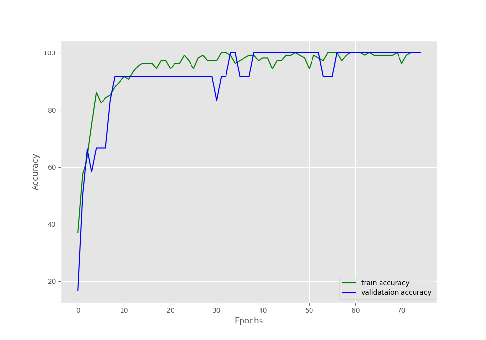
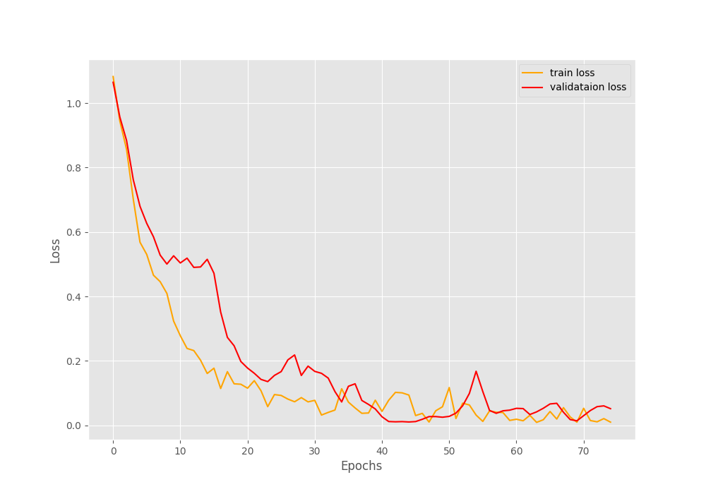
As you can see, the validation accuracy graph has plateaued long before the training completes. But the training accuracy and loss, both seem to be improving till the end of training. This shows how much difficult image augmentation has made the training set. This is one of the reasons also why we are able to train such a small dataset for so long without overfitting. Let’s hope that our model has learned well enough to give decent inference results.
The Inference Code
We will write the inference code in the inference.py script.
Starting with the import statements, defining a few constants, and loading the trained model.
import torch
import cv2
import numpy as np
import glob as glob
import os

from model import build_model
from torchvision import transforms

# Constants.
DATA_PATH = '../input/test_data'
IMAGE_SIZE = 224
DEVICE = 'cpu'

# Class names.
class_names = ['Bacterial leaf blight', 'Brown spot', 'Leaf smut']

# Load the trained model.
model = build_model(pretrained=False, fine_tune=False, num_classes=3)
checkpoint = torch.load('../outputs/model.pth', map_location=DEVICE)
print('Loading trained model weights...')
model.load_state_dict(checkpoint['model_state_dict'])
For the constants, we have the path to the test data, the image size to resize to, and the computation device. Then we define the class names on line 16 and load the pretrained model weights.
The next block of code contains two things:
- Capturing all the test image paths.
- A large
forloop which:- Iterates over the image paths.
- Extracts the ground truth label from the file name.
- Applies the preprocessing transform to the image.
- Predicts the output.
- Annotates the original image with the ground truth and the prediction.
- Shows the results on screen and saves it to disk.
# Get all the test image paths.
all_image_paths = glob.glob(f"{DATA_PATH}/*")

# Iterate over all the images and do forward pass.
for image_path in all_image_paths:
    # Get the ground truth class name from the image path.
    gt_class_name = image_path.split(os.path.sep)[-1].split('.')[0]
    # Read the image and create a copy.
    image = cv2.imread(image_path)
    orig_image = image.copy()

    # Preprocess the image
    image = cv2.cvtColor(image, cv2.COLOR_BGR2RGB)
    transform = transforms.Compose([
        transforms.ToPILImage(),
        transforms.Resize((IMAGE_SIZE, IMAGE_SIZE)),
        transforms.ToTensor(),
        transforms.Normalize(
            mean=[0.485, 0.456, 0.406],
            std=[0.229, 0.224, 0.225]
        )
    ])
    image = transform(image)
    image = torch.unsqueeze(image, 0)
    image = image.to(DEVICE)

    # Forward pass throught the image.
    outputs = model(image)
    outputs = outputs.detach().numpy()
    pred_class_name = class_names[np.argmax(outputs[0])]
    print(f"GT: {gt_class_name}, Pred: {pred_class_name.lower()}")
    # Annotate the image with ground truth.
    cv2.putText(
        orig_image, f"GT: {gt_class_name}",
        (10, 25), cv2.FONT_HERSHEY_SIMPLEX,
        0.8, (0, 255, 0), 2, lineType=cv2.LINE_AA
    )
    # Annotate the image with prediction.
    cv2.putText(
        orig_image, f"Pred: {pred_class_name.lower()}",
        (10, 55), cv2.FONT_HERSHEY_SIMPLEX,
        0.8, (100, 100, 225), 2, lineType=cv2.LINE_AA
    )
    cv2.imshow('Result', orig_image)
    cv2.waitKey(0)
    cv2.imwrite(f"../outputs/{gt_class_name}.png", orig_image)
With this, we are done with the inference code also. Let’s execute this script and see how well the model performs.
Executing inference.py
Execute the following command in the terminal/command line.
python inference.py
The following is the output from the terminal.
[INFO]: Not loading pre-trained weights
[INFO]: Freezing hidden layers...
Loading trained model weights...
GT: bacterial_leaf_blight, Pred: leaf smut
GT: leaf_smut, Pred: leaf smut
GT: brown_spot, Pred: brown spot
And the following are the image results.
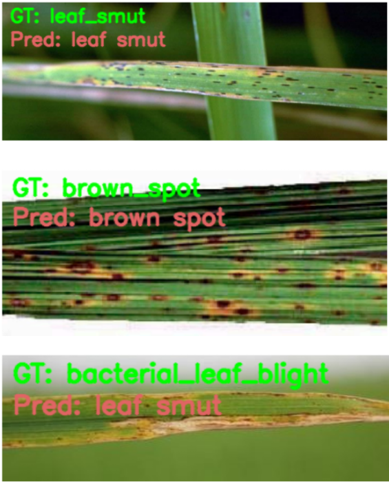
The model is able to predict brown spot and leaf smut classes correctly but not the baterial leaf blight. One of the reasons for this might be the difference in the background between the dataset images and the inference images. All the dataset images were placed on a white table, but it is not the case for all the inference images.
Further Experiments
There are quite a few things that can be added to this project.
- If you wish to do any improvement in the model here, more data is surely needed. Most probably, a better model cannot be trained with this amount of data.
- One of the other nice things can be done here is creating a small mobile app to recognize rice leaf diseases. This accompanying paper might be a good starting point.
If you carry out any of the above points, do let others know in the comment section.
Summary and Conclusion
In this post, you learned how to carry out rice leaf disease recognition using deep learning with a very small dataset. We used a lot of image augmentation techniques and a pretrained MobileNetV3 large model to achieve as good results as possible. I hope this post was helpful to you.
If you have any doubts, thoughts, or suggestions, please leave them in the comment section. I will surely address them.
You can contact me using the Contact section. You can also find me on LinkedIn, and X.
Image Credits
Following are the inference image credits:
brown_spot.png: Diseases of Rice.bacterial_leaf_blight.jpg: Forestry Images.leaf_smut.png: The Smuts (and non‐smuts) in Rice

Good content 🙂
Thank you.