
In this post, we will go in-depth into the understanding of Wide Residual Neural Networks. Also known as WRNs or Wide ResNets for short. We will go through the paper, the implementation details, the network architecture, the experiment results, and the benefits they provide.
When the original ResNet paper was published, it was a big deal in the world of deep learning. The residual blocks were very efficient for building deeper neural networks. Because of the residual blocks, residual networks were able to scale to hundreds and even thousands of layers and were still able to get an improvement in terms of accuracy. But even just stacking one residual block after the other does not always help. There are diminishing returns after a point. And this is where we need to take a look at something new.
To counter this issue and build even more efficient residual networks, now we have Wide Residual Neural Networks or WRN for short. We can also call them Wide ResNets. Wide Residual Neural Networks were introduced in the paper Wide Residual Networks by Sergey Zagoruyko and Nikos Komodakis. After publication, the paper has gone under a few revisions, and the current one is version 4 published in June 2017. Although the paper has a decent number of citations, still, many newcomers in deep learning may not get exposure to this paper. And hence, we will have a thorough discussion of the paper in this post.
We will cover the following topics here.
- General issues with original ResNets.
- Introduction to Wide Residual Networks.
- Architecture of Wide Residual Neural Networks.
- Experiments and results discussion.
- Forward and backward pass time comaparison between the original ResNet models and Wide ResNets.
Before Moving Further…
If you are already familiar with Wide ResNets and are aware of more details about it, you are very welcome to share your insights in the comment section. In case you find that this post misses something, then your viewpoints are very welcome.
If you are a beginner or going through the paper for the first time, I hope this provides new learning for you in the field of deep learning. Also, if you are learning about ResNets for the very first time here, I recommend that you go through the explanation of the original ResNets first. I am sure that would help.
That being said, let’s move ahead in this post.
General Issues with Original Residual Neural Networks
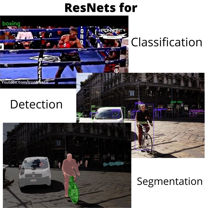
The original ResNets first came into the picture in 2015 in the paper Deep Residual Learning for Image Recognition by the authors Kaiming He, Xiangyu Zhang, Shaoqing Ren, and Jian Sun. ResNets became a baseline for many upcoming state-of-the-art neural networks in image classification, image segmentation, and object detection.
Because of the residual blocks, ResNets were able to show better generalization capabilities. This means they perform better in transfer learning in comparison to other networks of the same scale and number of parameters.
But the main focus to improving the accuracy of ResNets was by adding more and more residual blocks to increase the depth of the network. There came a point where deeper residual blocks give diminishing results.
As mentioned in the Wide Residual Network, when a ResNet is thousands of layers deep, there are a few problems we face.
- Each fraction of improvement in performance costs double the number of layers.
- Very deep residual networks (those having thousands of layers) have a dimishing return for feature reuse. This means that they may not be just as fast to converge. And even may not be helpful for transfer learning.
The above two problems directly tell that just building deeper networks even with residual blocks will not help.
Introduction to Wide Residual Neural Networks
With the above two problems to tackle, Sergey Zagoruyko and Nikos Komodakis came up with Wide Residual Neural Networks.
In the paper, they propose a new way of using the residual blocks for building Residual Neural Networks. They try to decrease the depth of the networks and increase the width.
They take the same residual block concept from the original ResNets and try to increase the width of each block. What does increasing the width mean? For each convolutional layer in the residual block, they add more kernels. They even experiment with dropouts in-between the convolutional layers which have their own potential.
With the above changes and other improvements, the authors are able to achieve much better results. A 16 layer deep Wide Residual Neural Network is able to beat an original ResNet with hundreds or even thousands of layers.
A Simple Comparison with Original ResNets
The original ResNets were thin and deep and even had bottleneck layers to reduce parameters. The authors of Wide ResNets argue that such depth also became a weakness for the original ResNets. They mention the issue in the paper which I am quoting here.
As gradient flows through the network there is nothing to force it to go through residual block weights and it can avoid learning anything during training, so it is possible that there is either only a few blocks that learn useful representations, or many blocks share very little information with small contribution to the final goal. This problem was formulated as diminishing feature reuse…
Wide Residual Networks, Sergey Zagoruyko and Nikos Komodakis
Wide ResNets with less depth and more width can have 50 times fewer layers than the original ResNets. At the same time, they are 2 times faster to train. This type of wide network with just a few tens of layers can provide better results than a 1000 layer deep original ResNet.
Contributions of Wide Residual Networks
Before getting into the architecture details of Wide ResNets, let’s take a look at the main contributions of the paper.
- The authors present a number of experiments using the Residual block structure. This can help in future experiments and even building better neural networks.
- The Wide ResNets in the paper provide better performance and faster training compared to previous deep networks.
- We also see a new way of using dropouts to prevent overfitting.
- The new Wide ResNets provide better training results on many benchmark datasets. They also train faster when compared to previous Residual neural networks.
Architecture of Wide Residual Neural Networks
The Wide ResNets essentially follow a similar architecture to the original ResNets with a unique naming convention. We can identify a Wide ResNet by naming it as WRN-n-k. Here, n refers to the total number of convolutional layers and k refers to the widening factor.
So, when we say WRN-40-2, it is a Wide ResNet with 40 layers and 2 as the widening factor. Whenever the widening factor k=1, the network follows the original “thin” ResNet structure. Whenever the widening factor k>2, the network follows the Wide ResNet structure.
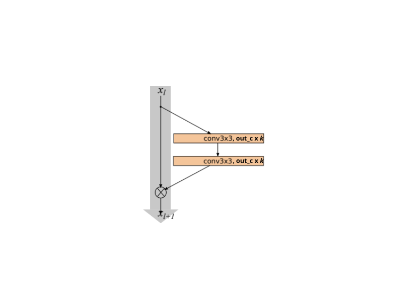
One question that arises here, how to use the widening factor k? Well, we simply multiply k with the number of output kernels of that particular convolutional layer. So, for Wide ResNet, a general residual block with a widening factor will look like the following.
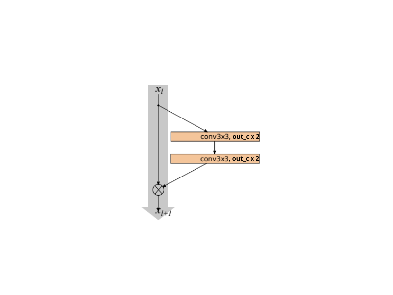
And if the widening factor is k=2, we simply multiply it.
The General Structure of Wide Residual Neural Networks
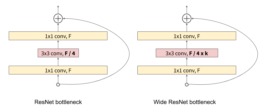
In the original ResNets, there were two types of residual blocks:
- The basic residual block: Consisting of two consecutive 3×3 convolutional layers preceded by batch normalizaton and ReLU non-linearity. It is
conv3x3-conv3x3. - The bottleneck block: Here, dimensionality reducing and expanding 1×1 convolutions surround a 3×3 convoltional layer. It is
conv1×1-conv3×3-conv1×1.
The bottleneck layer’s main work is to make the network less computationally expensive. Also, it helps to make the network deeper. But as the aim of Wide ResNets is to make the network wider instead of deeper, the authors of Wide ResNets avoid it.
With that, the following is the general structure of a Wide Residual Neural Network.
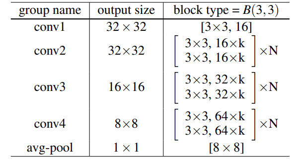
There are a few things to observe here.
- The brackets show the groups of convolution where k determines the width of the network.
- There are 4 groups of convolution, where N determines the number of blocks in a particular group.
- The above structure does not show the final classification layer for clarity.
One more thing to note here is the block type = B(3,3). This shows the type of convolutional layers used in the block. B(3, 3) means that it contains 3×3 convolutional layers. This is important because the authors experiment with all the following block types.

The authors also experiment with the number of convolutional layers per block and the number of blocks in the entire network itself. The number of the convolutional layers in each block is controlled by a deepening factor called l. And d denotes the number of blocks in the entire network.
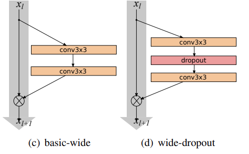
Use of Dropout in Residual Blocks
In deep neural networks, we generally use dropouts in the fully-connected layers to reduce the number of parameters. For the Wide ResNets, the authors introduce dropouts between the convolutional layers in the residual blocks.

This has the potential to:
- Reduce overfitting while training.
- Helps in mitigating the issue of diminishing feature reuse when the network depth is more.
Further, according to the authors, this provides improved gains in accuracy of the network that can lead to new state-of-the-art results.
Experiments and Results
In this section, we move on to discuss the experiments and results carried by the authors using Wide ResNets.
The authors chose CIFAR-10, CIFAR-100, SVHN, and ImageNet datasets for image classification experiments. And the COCO dataset was chosen for object detection experiments.
CIFAR10, CIFAR100, and SVHN Experiments
Let’s start with the results from the image classification experiments. These experiments follow a standard set of preprocessing and settings for each dataset.
- For the CIFAR10 and CIFAR100 datasets, the authors use horizontal flips and random crop as data augmentation. Furthermore, they also use ZCA whitening as one of the preprocessings.
- And for the SVHN dataset, the authors only divide the images by 255 to make the pixel range [0, 1].
Going through Section 3 of the paper in detail will provide a few more information. These include types of convolutions, the number of convolutions per block, and the width of the residual blocks. Here, we will just focus on the results part a bit more.
Comparison with Original ResNets
The following figure of tabulated results shows the information about CIFAR10 and CIFAR100 datasets.

As we can see, WRN-28-10 and WRN-28-12 achieve low test error on CIFAR10 and CIFAR100 datasets respectively. But how do they compare to the other deep neural networks and especially to the original ResNets?
The following results from the paper show a much better comparison.

It is clear that WRN-28-10 is easily beating the original ResNets consisting of even more than 1000 layers. And if you see, these test errors for WRN-28-10 here are a bit lower than the previous one. This might be because of flip and translation data augmentations along with mean/std normalization.
There is one concern that arises here though. We are comparing a 36 million parameters Wide ResNet model with a 10 million parameters original ResNet model. How do we know it is not just the increase in parameters that are helping? In that case, we can compare the original ResNet with WRN 40-4 with around 9 million parameters. Even this is giving less test error than the original ResNets.
Even the following graphs show that Wide ResNets give less error when compared with other original ResNet structures.

In the above figure, the solid lines denote the test error, and dashed lines denote the training loss. In both cases, Wide Residual Neural Networks seem to be performing better.
Effect of Dropout in Residual Blocks
Earlier we discussed that the authors used dropouts between the convolutional layers in the residual blocks of Wide ResNets. This is not very common as we generally add dropouts after the fully-connected layers.
With this approach, the results improved even further.

Observing the above results tell us that the same WRN-28-10 model now achieves even lower error rates of 3.89 and 18.85 on CIFAR10 and CIFAR100 respectively.
We can say the same for results on the SVHN dataset as well.
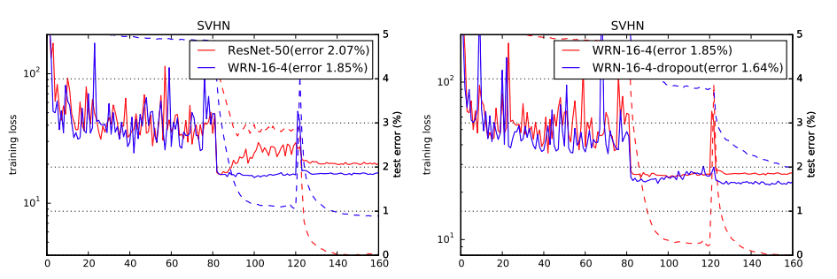
Here, WRN-16-4 is already beating a ResNet50 model without using dropout. And adding dropout only improves the results.
Not just the Wide Residual Neural Networks, even the original ResNets improve by using dropouts in the residual blocks. The following lines from the authors confirm this.
We observe significant improvements from using dropout on both thin and wide networks. Thin 50-layer deep network even outperforms thin 152-layer deep network with stochastic depth.
Wide Residual Networks, Sergey Zagoruyko and Nikos Komodakis
ImageNet and COCO Experiments
Now, let’s discuss the final set of experiments for the Wide Residual Neural Networks. Those are the ImageNet classification and COCO object detection experimental results.
Here, the experiments and comparison include both bottleneck and non-bottleneck networks. And this is the case for both the original ResNets and the Wide ResNets. Previously, the authors had planned that the bottleneck layers will not be used in the Wide Residual Networks. However, here they find that the ResNets and Wide ResNets with bottleneck layers outperform non-bottleneck networks. They conclude that the bottleneck networks might just be better suited for the ImageNet classification task. Or as ImageNet is a very complex classification task, it simply needs deeper neural networks.
On ImageNet
For the ImageNet experiments, the authors modified the original ResNet architectures to make them wider. We start with the ResNet-50 network and make the 3×3 residual connections wider by a factor of 2.0. Here, we observe this wide network outperforms a ResNet-152 network having 3 times the less number of layers. Not only that, WRN-50-2 trains much faster than the ResNet-152 network.
But the WRN-50-2 network performs a bit worse when compared to the ResNet-200 network under the same ImageNet training settings. The following image shows all the results on the ImageNet dataset.
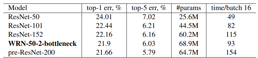
The above results show the validation error on the ImageNet dataset.
COCO Dataset and Other Cumulative Results
For the COCO training, the authors use a WRN-34-2. But they also use techniques from MultiPathNet and LocNet. The following image of the table from the paper contains the best results for Wide Residual Neural Networks.
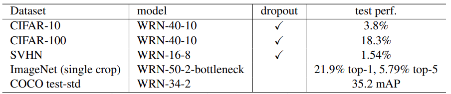
At the time of publication, these COCO results of 35.2 mAP were the best single model performance. Here, the WRN-34-2 for COCO uses VGG-16-based AttractioNet proposals and has a LocNet-style localization part. Also, the CIFAR10, CIFAR100, and SVHN results were the best results for single runs at the time of publication.
Forward and Backward Pass Time Comparison
Not just the training convergence time, the Wide ResNets also appear to be faster in the forward+backward pass time. When compared with their thin ResNet counterparts, WRNs show better GPU computational efficiency.
The following results were benchmarked with cuDNN version 5 and a Titan X GPU.
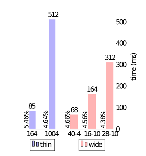
These results are from training on the CIFAR10 dataset. The percentages beside the bar plots show the test error. Here, the WRN-28-10 is about 1.6 times faster than the thin ResNet-1001. And the WRN-40-4 having almost the same accuracy as ResNet-1001 is around 8 times faster.
Final Remarks
All in all, Wide Residual Neural Networks show good potential in image classification and also object detection when used in combination with other techniques. The benchmark dataset results show them to be better than the thin ResNets in many aspects. However, maybe more real-world dataset results are also needed before we can conclude something concretely. Hopefully, we will be able to explore that aspect in future posts and tutorials.
You can get all the training settings and implementation details under the Implementation details heading in the paper. Here, you can find the official GitHub repository and code. And one of the best things. They have their pretrained neural networks on PyTorch Hub that you can try right away. Also, previously, I had written a post comparing the forward pass time of Wide ResNet and original ResNets which you can find here. It uses the PyTorch Hub model.
Summary and Conclusion
In this post, we explored the Wide ResNet paper in detail. We went over the contributions, the architecture, the experiments, and the results. If you find that anything is missing or perhaps misleading, please notify as such in the comment section. I hope that you learned something new from this post.
If you have any doubts, thoughts, or suggestions, please leave them in the comment section. I will surely address them.
You can contact me using the Contact section. You can also find me on LinkedIn, and X.

1 thought on “Wide Residual Neural Networks – WRNs: Paper Explanation”