Training a Custom PyTorch Classifier on Medical MNIST Dataset

In this tutorial, we will classify images from the Medical MNIST dataset. In fact, we will be training a custom PyTorch classifier on the Medical MNIST dataset.

Recently, deep learning has been sweeping into many different industries. It’s helping to solve problems that were thought to be impossible to solve before. Computer vision, in particular, is helping different industries like manufacturing, automobile, surveillance, and security. It’s helping to create insights and future predictions using the huge amount of data they produce. And healthcare is no different. Deep learning is here as well. Starting from classifying whether a person has a tumor or not or predicting whether a person might get skin cancer in the future. Deep learning is helping to solve different healthcare problems.

Especially during the COVID-19 pandemic, deep learning became a big help in detecting whether a person is wearing a mask or not. And even classifying whether a person has COVID-19 or not. All of this is possible because of computer vision and deep learning.

What Will We Cover Here?

Although we will not be tackling problems as difficult as mentioned above, we will do the best we can on the dataset that we have. Before going into the technical details of the post, let’s take a look at the points that we will be covering in this tutorial.

• We will start with the exploration of the Medical MNIST dataset from Kaggle.
• Then we will move on to the preparation of the dataset. Although the data is available in pretty good format, we will change it’s directory structure a bit.
• Next, we will jump into the deep learning coding part. Starting with the helper functions, data loader preparation, writing the custom model, till training, we will cover all. All of this will help us in training the custom PyTorch classifier on the Medical MNIST dataset.
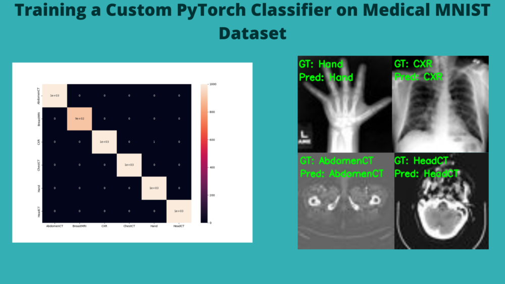
• After training the PyTorch classifier on the Medical MNIST dataset and saving the model to disk, we will also run testing on a held-out set. This will help us know the capability of our model much better. Along with visualizing a few test images, we will also plot the confusion matrix for much clearer understanding of our model’s performace.
• Finally, we will discuss how to take this simple project even further.

This is going to be an exciting post. Let’s jump into it now.

The Medical MNIST Dataset

We will use the Medical MNIST dataset from Kaggle for training our custom PyTorch image classifier. You might already be familiar with the Digit MNIST and Fashion MNIST datasets. These two datasets are commonly used to teach the basic concepts of deep learning to beginners. It is also not uncommon to try out any new deep learning model/architecture on these datasets to check out the performance. Although other datasets are replacing these two for such benchmarks. In short, the Digit MNIST dataset contains 28×28 grayscale images of digits from 0 to 9. And the Fashion MNIST dataset contains 28×28 grayscale images of fashion products.

The Medical MNIST dataset is similar with a few changes. It contains medical images in the MNIST-style. This means that all the images are 64×64 grayscale images.

Number of Images and Classes

The Medical MNIST dataset contains 58954 images of 64×64 dimensions. All the images are in grayscale format and there are 6 classes in total. They are:

• AbdomenCT – 10000 images
• BreastMRI – 8954 images
• CXR (Chest X-Ray) – 10000 images
• ChestCT – 10000 images
• Hand – 10000 images
• HeadCT – 10000 images

You can also find the original dataset here on GitHub along with a few companion notebooks.

Our Approach to the Medical MNIST Classification Problem

If you go through the dataset structure on Kaggle, you will notice that all the images are in the respective class folders. This is good enough. However, we will change the dataset structure a bit. We will divide the data into 70% training, 20% validation, and 10% test set. We may call it a simple data preparation step and all the code will be available along with this tutorial.

While training, we will go through the particular image and hyperparameter settings. For now, you can download the dataset from here that we will use further on.

Directory Structure

Let’s check out the directory structure for this project.

├── input
│   ├── medical_mnist
│   │   ├── AbdomenCT [10000 entries exceeds filelimit, not opening dir]
│   │   ├── BreastMRI [8954 entries exceeds filelimit, not opening dir]
│   │   ├── ChestCT [10000 entries exceeds filelimit, not opening dir]
│   │   ├── CXR [10000 entries exceeds filelimit, not opening dir]
│   │   ├── Hand [10000 entries exceeds filelimit, not opening dir]
│   │   └── HeadCT [10000 entries exceeds filelimit, not opening dir]
│   └── medical_mnist_processed
│       ├── test
│       │   ├── AbdomenCT [1000 entries exceeds filelimit, not opening dir]
│       │   ├── BreastMRI [895 entries exceeds filelimit, not opening dir]
│       │   ├── ChestCT [1000 entries exceeds filelimit, not opening dir]
│       │   ├── CXR [1000 entries exceeds filelimit, not opening dir]
│       │   ├── Hand [1000 entries exceeds filelimit, not opening dir]
│       │   └── HeadCT [1000 entries exceeds filelimit, not opening dir]
│       ├── train
│       │   ├── AbdomenCT [7000 entries exceeds filelimit, not opening dir]
│       │   ├── BreastMRI [6267 entries exceeds filelimit, not opening dir]
│       │   ├── ChestCT [7000 entries exceeds filelimit, not opening dir]
│       │   ├── CXR [7000 entries exceeds filelimit, not opening dir]
│       │   ├── Hand [7000 entries exceeds filelimit, not opening dir]
│       │   └── HeadCT [7000 entries exceeds filelimit, not opening dir]
│       └── valid
│           ├── AbdomenCT [2000 entries exceeds filelimit, not opening dir]
│           ├── BreastMRI [1790 entries exceeds filelimit, not opening dir]
│           ├── ChestCT [2000 entries exceeds filelimit, not opening dir]
│           ├── CXR [2000 entries exceeds filelimit, not opening dir]
│           ├── Hand [2000 entries exceeds filelimit, not opening dir]
│           └── HeadCT [2000 entries exceeds filelimit, not opening dir]
├── notebooks
│   └── process_medical_mnist.ipynb
├── outputs
│   ├── accuracy.png
│   ├── heatmap.png
│   ├── loss.png
│   ├── model.pth
│   ├── test_image_1998.png
│   ├── test_image_2997.png
│   ├── test_image_3996.png
│   ├── test_image_4995.png
│   └── test_image_999.png
└── src
    ├── datasets.py
    ├── model.py
    ├── test.py
    ├── train.py
    └── utils.py

Okay! there are quite a few things to cover here. Moving over each directory at a time.

• input: The medical_mnist directory here contains the original dataset that we obtain after downloading and extracting it from Kaggle. However, we can also see a medical_mnist_processed directory. This contains the dataset that has been split into train, valid, and test directories with 70%, 20%, 10% data respectively. But how do we obtain this data? Taking a look at the next directory will help us uncover that.
• notebooks: This directory contains a single notebook, that is, process_medical_mnist.ipynb. It contains the code that will generate the data present in medical_mnist_processed. We don’t have to go through the details of the code in this notebook. Just noting that running this notebook generates the required data for us is enough.
• outputs: As the name suggests, this directory will contain the model and accuracy & loss graphs from training. Along with that, it will also hold the confusion matrix and a few resulting test images from the testing phase.
• src: This contains three Python files. We will discuss the details of these while writing the code.

As of now, it is much better if you download the zip file for this tutorial. This contains all the code including the notebook for preparing the data. Separately, you need to download the data from Kaggle and place it in the appropriate directory after extracting and renaming it.

PyTorch Version and Other Libraries

All the code in this tutorial has been developed using PyTorch 1.10.0. Although a slightly older version and newer versions as well should not cause any issues.

If you need to download/upgrade your PyTorch version, you can do so from here.

Also, please ensure that you have Scikit-Learn and Seaborn installed in your working environment. We will need these while testing the model.

Training a Custom PyTorch Image Classifier on the Medical MNIST Dataset

Now, we will jump into the coding part of this tutorial. There are a few things to take care of first. We will cover the coding part in the following order.

• First, we will execute the code in the process_medical_mnist.ipynb in the notebooks directory to generate the data for our use. This data will be stored in the input/medical_mnist_processed directory.
• Moving on to the Python files, we will write a few helper functions in utils.py.
• Then we will write the code in datasets.py to prepare the datasets and data loaders.
• Next, we will prepare the neural network model whose code will go into model.py.
• The training code will go into train.py. This is the executable script that will run training and validation.
• After we have the trained model, we will use it to run a final test on the held-out set. This code will go into the test.py script.

Although this seems long, training a custom PyTorch image classifier on the Medical MNIST dataset is going to be pretty fun.

Executing the Code in process_medical_mnist.ipynb to Generate the Required Data

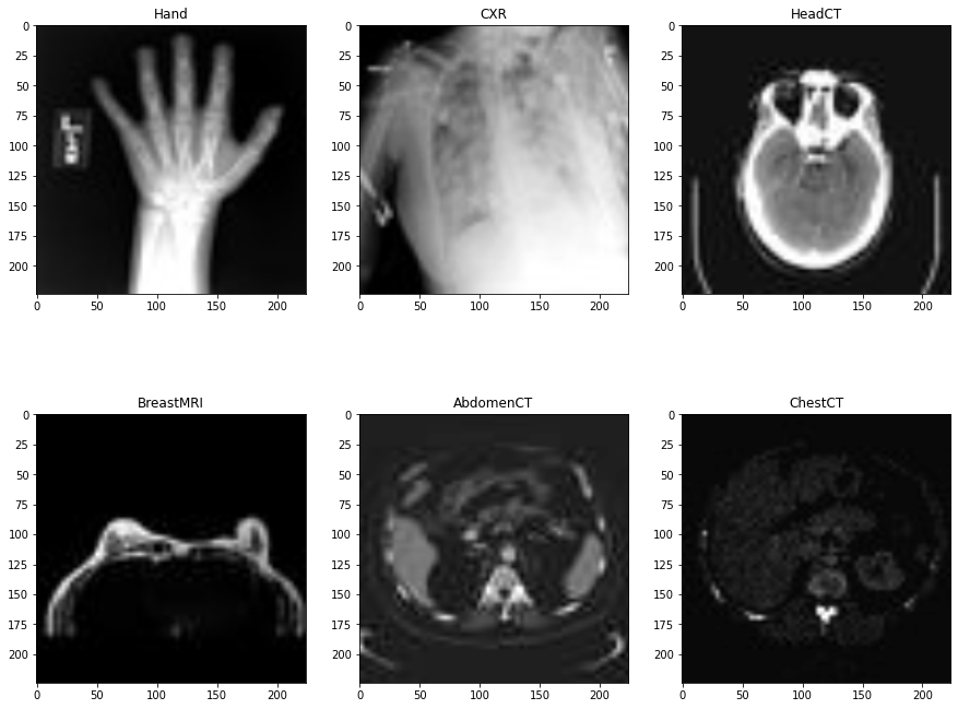
This is the first step that we will go through. That is executing the code in process_medical_mnist.ipynb to generate the data in medical_mnist_processed directory. We will not go through this processing code here. If you go through the notebook, you will find that the preprocessing code is pretty simple and straightforward. It visualizes a few images and splits the original data into training, validation, and test sets.

Before executing the code in process_medical_mnist.ipynb please ensure that you have created the medical_mnist_processed subdirectory inside the input directory. The processing should be complete within a few seconds only.

Writing the Helper Function

Now, let’s write a few helper functions to ease out a few tasks while we train the model. There are two functions, one for saving the trained model, and the other one for saving the loss and accuracy graphs.

The code here will go into the utils.py file.

Starting with the import statements and the function to save the trained model.

import torch
import matplotlib
import matplotlib.pyplot as plt

matplotlib.style.use('ggplot')

def save_model(epochs, model, optimizer, criterion):
    """
    Function to save the trained model to disk.
    """
    torch.save({
                'epoch': epochs,
                'model_state_dict': model.state_dict(),
                'optimizer_state_dict': optimizer.state_dict(),
                'loss': criterion,
                }, f"../outputs/model.pth")

The above function will save the trained model to disk. It saves the model state dictionary, the number of epochs trained for, the optimizer state dictionary, and also the loss function. This will help to resume training in the future if we intend to do so.

Next, the function to save the accuracy and loss plots.

def save_plots(train_acc, valid_acc, train_loss, valid_loss):
    """
    Function to save the loss and accuracy plots to disk.
    """
    # Accuracy plots
    plt.figure(figsize=(10, 7))
    plt.plot(
        train_acc, color='green', linestyle='-', 
        label='train accuracy'
    )
    plt.plot(
        valid_acc, color='blue', linestyle='-', 
        label='validataion accuracy'
    )
    plt.xlabel('Epochs')
    plt.ylabel('Accuracy')
    plt.legend()
    plt.savefig(f"../outputs/accuracy.png")
    
    # Loss plots
    plt.figure(figsize=(10, 7))
    plt.plot(
        train_loss, color='orange', linestyle='-', 
        label='train loss'
    )
    plt.plot(
        valid_loss, color='red', linestyle='-', 
        label='validataion loss'
    )
    plt.xlabel('Epochs')
    plt.ylabel('Loss')
    plt.legend()
    plt.savefig(f"../outputs/loss.png")

The save_plots() function simply accepts the lists containing the training accuracy, validation accuracy, training loss, and validation loss values. Then it uses matplotlib to save the graphs to disk.

Preparing the Medical MNIST Dataset

Now, we will prepare the Medical MNIST datasets and data loaders. We already have all the dataset splits in the medical_mnist_processed directory. So, we can use the ImageFolder to create the datasets easily.

The dataset preparation code will go into the datasets.py file.

The first code block for dataset preparation contains the import statements and a few constants.

from torchvision import datasets, transforms
from torch.utils.data import DataLoader

# Required constants.
TRAIN_DIR = '../input/medical_mnist_processed/train'
VALID_DIR = '../input/medical_mnist_processed/valid'
IMAGE_SIZE = 224 # Image size of resize when applying transforms.
BATCH_SIZE = 64
NUM_WORKERS = 4 # Number of parallel processes for data preparation.

Going over the contents:

• We are defining the training and validation directory paths as TRAIN_DIR and VALID_DIR. Note that we are not using the test data here. That will be used after training and validation for the final testing.
• The IMAGE_SIZE constant defines the dimensions that the images will be resized while applying the transformations. Remember that the original images are 64×64 in dimension, but we will be resizing them to 224×224 here. Though the images will get a bit blurry there is a very high chance that the model will still be able to extract more fine-grained features from larger image sizes. Also, it is worth noting that larger image sizes will take longer to train. So, if you are training on your local system and training time is too long, try training with the original 64×64 dimensions.
• Next is the batch size. In the current code it is 64. If you face OOM (Out Of Memory) error because of large batch size, try reducing to either 32, 16, or even 8. Again, when you change the batch size, your might need to train for less or more number of epochs to obtain the same accuracy as we do here. This is a setting to experiment with.
• Finally, we set the number of parallel workers for the dataset transform/preprocessing part. It is set to 4 and most modern processors should support this.

The Training and Validation Transforms

We will use transforms from torchvision to apply the preprocessing and augmentation transforms. Let’s write the code for that first.

# Training transforms
def get_train_transform(IMAGE_SIZE):
    train_transform = transforms.Compose([
        transforms.Resize((IMAGE_SIZE, IMAGE_SIZE)),
        transforms.RandomHorizontalFlip(p=0.5),
        transforms.GaussianBlur(kernel_size=(5, 9), sigma=(0.1, 5)),
        transforms.RandomAdjustSharpness(sharpness_factor=2, p=0.5),
        transforms.ToTensor(),
        transforms.Normalize(
            mean=[0.5, 0.5, 0.5],
            std=[0.5, 0.5, 0.5]
            )
    ])
    return train_transform

# Validation transforms
def get_valid_transform(IMAGE_SIZE):
    valid_transform = transforms.Compose([
        transforms.Resize((IMAGE_SIZE, IMAGE_SIZE)),
        transforms.ToTensor(),
        transforms.Normalize(
            mean=[0.5, 0.5, 0.5],
            std=[0.5, 0.5, 0.5]
            )
    ])
    return valid_transform

There are a few important things to note here:

• First, we have the get_train_transform() function which returns the training transforms and augmentations. It accepts the image resizing value as the parameter. For augmentations, we are randomly flipping the images horizontally, applying Gaussian blur, and adjusting the sharpness randomly. There are many more augmentations that we can apply here. Still, we need to be a bit careful as we should not apply just any random augmentation to medical images. If you apply any more augmentation, be a bit careful that the augmented image should retain it’s inherent properties as a medical image should.
• For the validation transform, we just apply the general preprocessing and no augmentations.
• Coming to the important point now. If you observe the normalization, you will see that we are applying it across three channels. If you remember, our original dataset is in grayscale format. So, why apply across three channels? The reason lies how ImageFolder class prepares the dataset. It uses PIL internally and also converts every image to RGB format. So, our single channel grayscale images have now become three channel grayscale images. It is better to keep this point in mind as we need to prepare the neural network model according to the input image channels.

Functions to Prepare the Datasets and Data Loaders

For the final part of the dataset preparation, we will write simple functions for preparing the datasets and data loaders.

def get_datasets():
    """
    Function to prepare the Datasets.

    Returns the training and validation datasets along 
    with the class names.
    """
    dataset_train = datasets.ImageFolder(
        TRAIN_DIR, 
        transform=(get_train_transform(IMAGE_SIZE))
    )
    dataset_valid = datasets.ImageFolder(
        VALID_DIR, 
        transform=(get_valid_transform(IMAGE_SIZE))
    )
    return dataset_train, dataset_valid, dataset_train.classes

def get_data_loaders(dataset_train, dataset_valid):
    """
    Prepares the training and validation data loaders.

    :param dataset_train: The training dataset.
    :param dataset_valid: The validation dataset.

    Returns the training and validation data loaders.
    """
    train_loader = DataLoader(
        dataset_train, batch_size=BATCH_SIZE, 
        shuffle=True, num_workers=NUM_WORKERS
    )
    valid_loader = DataLoader(
        dataset_valid, batch_size=BATCH_SIZE, 
        shuffle=False, num_workers=NUM_WORKERS
    )
    return train_loader, valid_loader 

The get_datasets() function prepares the training and validation datasets and returns them along with the dataset class names.

The get_data_loaders() function accepts the training and validation datasets. It prepares the data loaders and returns them. As all our preprocessing functions and constants are already defined, here we just provide the required arguments.

This completes the dataset preparation code. While most of it was straightforward, we went over a few important details as well.

The PyTorch Neural Network Classifier for Medical MNIST Classification

It’s time to write the code to prepare the neural network model now. It is going to be a very simple convolutional network.

The neural network model preparation code will go into the model.py file.

The following code block contains the entire network architecture code.

import torch.nn.functional as F
import torch.nn as nn

class MedicalMNISTCNN(nn.Module):
    def __init__(self, num_classes=None):
        super(MedicalMNISTCNN, self).__init__()
        self.conv_block = nn.Sequential(
            nn.Conv2d(in_channels=3, out_channels=32, kernel_size=3),
            nn.ReLU(),
            nn.MaxPool2d(kernel_size=2, stride=2),
            nn.Conv2d(in_channels=32, out_channels=64, kernel_size=3),
            nn.ReLU(),
            nn.MaxPool2d(kernel_size=2, stride=2),
            nn.Conv2d(in_channels=64, out_channels=128, kernel_size=3),
            nn.ReLU(),
            nn.MaxPool2d(kernel_size=2, stride=2),
            nn.Conv2d(in_channels=128, out_channels=256, kernel_size=3),
            nn.ReLU(),
            nn.MaxPool2d(kernel_size=2, stride=2)
        )

        self.classifier = nn.Sequential(
            nn.Linear(in_features=256, out_features=128),
            nn.Dropout2d(p=0.4),
            nn.Linear(in_features=128, out_features=num_classes)
        )

    def forward(self, x):
        x = self.conv_block(x)
        bs, _, _, _ = x.shape
        x = F.adaptive_avg_pool2d(x, 1).reshape(bs, -1)
        x = self.classifier(x)
        return x

The model consists of two Sequential blocks, the feature extractor, self.conv_block, and the classifier, self.classifier.

For the feature extraction part (starting from line 7), we use a simple stacking of convolutional layers, ReLU activation, and 2D max-pooling layers.

For the classification head (starting from line 22), we have a Linear => Dropout => Linear structure.

From line 28, we have the forward() function which passes the tensors through the layers and returns the final outputs (logits). Note that we are using adaptive_avg_pool2d layer instead of flattening the convolutional features. This has two benefits. It will help reduce the number of parameters in the model and also allow us to resize images (if needed) while data preparation without worrying about the model’s classifier part.

With this, we complete the model preparation code as well.

The Training Script

Before we can begin training our PyTorch image classifier on the Medical MNIST dataset, we need to prepare the training script. This will basically connect all the parts together that we have been preparing and run the training & validation loops.

We will write the code for the training script in train.py file.

The following code block contains the import statement and the construction of the argument parser.

import torch
import argparse
import torch.nn as nn
import torch.optim as optim
import time

from tqdm.auto import tqdm

from model import MedicalMNISTCNN
from datasets import get_datasets, get_data_loaders
from utils import save_model, save_plots

# Construct the argument parser.
parser = argparse.ArgumentParser()
parser.add_argument(
    '-e', '--epochs', type=int, default=10,
    help='Number of epochs to train our network for'
)
parser.add_argument(
    '-lr', '--learning-rate', type=float,
    dest='learning_rate', default=0.001,
    help='Learning rate for training the model'
)
args = vars(parser.parse_args())

We are importing all our custom modules which include the datasets, utils, and model.

For the argument parser, we have two flags.

• --epochs: To control the number of epochs to train for.
• --learning-rate: The learning rate for the optimizer.

The Training and Validation Functions

The training and validation functions that we will use here are pretty simple. We will just calculate the accuracy and loss functions after each epoch for the entire dataset. But when dealing with medical images, it is always better to calculate other metrics like precision, recall, and f1-score. We are not doing that here to keep things a bit simple. We will surely explore those in future articles.

The following block contains the training function.

# Training function.
def train(model, trainloader, optimizer, criterion):
    model.train()
    print('Training')
    train_running_loss = 0.0
    train_running_correct = 0
    counter = 0
    for i, data in tqdm(enumerate(trainloader), total=len(trainloader)):
        counter += 1
        image, labels = data
        image = image.to(device)
        labels = labels.to(device)
        optimizer.zero_grad()
        # Forward pass.
        outputs = model(image)
        # Calculate the loss.
        loss = criterion(outputs, labels)
        train_running_loss += loss.item()
        # Calculate the accuracy.
        _, preds = torch.max(outputs.data, 1)
        train_running_correct += (preds == labels).sum().item()
        # Backpropagation
        loss.backward()
        # Update the weights.
        optimizer.step()
    
    # Loss and accuracy for the complete epoch.
    epoch_loss = train_running_loss / counter
    epoch_acc = 100. * (train_running_correct / len(trainloader.dataset))
    return epoch_loss, epoch_acc

The training function iterates over the training data loader and returns the accuracy and loss for each epoch.

Now, the validation function.

# Validation function.
def validate(model, testloader, criterion):
    model.eval()
    print('Validation')
    valid_running_loss = 0.0
    valid_running_correct = 0
    counter = 0
    with torch.no_grad():
        for i, data in tqdm(enumerate(testloader), total=len(testloader)):
            counter += 1
            
            image, labels = data
            image = image.to(device)
            labels = labels.to(device)
            # Forward pass.
            outputs = model(image)
            # Calculate the loss.
            loss = criterion(outputs, labels)
            valid_running_loss += loss.item()
            # Calculate the accuracy.
            _, preds = torch.max(outputs.data, 1)
            valid_running_correct += (preds == labels).sum().item()
        
    # Loss and accuracy for the complete epoch.
    epoch_loss = valid_running_loss / counter
    epoch_acc = 100. * (valid_running_correct / len(testloader.dataset))
    return epoch_loss, epoch_acc

It is almost similar to the training function. But we do not need any backpropagation for validation.

The Main Code Block

The training will happen inside the if __name__ == '__main__' block. This is mainly to ensure that the training loop will only run if the training script is executed.

if __name__ == '__main__':
    # Load the training and validation datasets.
    dataset_train, dataset_valid, dataset_classes = get_datasets()
    print(f"[INFO]: Number of training images: {len(dataset_train)}")
    print(f"[INFO]: Number of validation images: {len(dataset_valid)}")
    print(f"[INFO]: Class names: {dataset_classes}\n")
    # Load the training and validation data loaders.
    train_loader, valid_loader = get_data_loaders(dataset_train, dataset_valid)

    # Learning_parameters. 
    lr = args['learning_rate']
    epochs = args['epochs']
    device = ('cuda' if torch.cuda.is_available() else 'cpu')
    print(f"Computation device: {device}")
    print(f"Learning rate: {lr}")
    print(f"Epochs to train for: {epochs}\n")

    model = MedicalMNISTCNN(num_classes=len(dataset_classes)).to(device)
    
    # Total parameters and trainable parameters.
    total_params = sum(p.numel() for p in model.parameters())
    print(f"{total_params:,} total parameters.")
    total_trainable_params = sum(
        p.numel() for p in model.parameters() if p.requires_grad)
    print(f"{total_trainable_params:,} training parameters.")

    # Optimizer.
    optimizer = optim.Adam(model.parameters(), lr=lr)
    # Loss function.
    criterion = nn.CrossEntropyLoss()

    # Lists to keep track of losses and accuracies.
    train_loss, valid_loss = [], []
    train_acc, valid_acc = [], []
    # Start the training.
    for epoch in range(epochs):
        print(f"[INFO]: Epoch {epoch+1} of {epochs}")
        train_epoch_loss, train_epoch_acc = train(model, train_loader, 
                                                optimizer, criterion)
        valid_epoch_loss, valid_epoch_acc = validate(model, valid_loader,  
                                                    criterion)
        train_loss.append(train_epoch_loss)
        valid_loss.append(valid_epoch_loss)
        train_acc.append(train_epoch_acc)
        valid_acc.append(valid_epoch_acc)
        print(f"Training loss: {train_epoch_loss:.3f}, training acc: {train_epoch_acc:.3f}")
        print(f"Validation loss: {valid_epoch_loss:.3f}, validation acc: {valid_epoch_acc:.3f}")
        print('-'*50)
        
    # Save the trained model weights.
    save_model(epochs, model, optimizer, criterion)
    # Save the loss and accuracy plots.
    save_plots(train_acc, valid_acc, train_loss, valid_loss)
    print('TRAINING COMPLETE')

First, we prepare the datasets and the data loader. Then we define all the learning parameters from line 92. After that, we initialize the model on line 99. After defining the optimizer and loss function (criterion), the training loop starts from line 117. As the training completes, we save the trained model and the accuracy & loss graphs to disk.

We are now all set to start the training procedure.

Executing train.py to Train the Neural Network Model

To start the training, open your command line/terminal in the src directory and execute the following command.

python train.py --epochs 20

We are training the model for 20 epochs with the default learning rate of 0.001. Depending on the hardware that you have, the training may take some time to complete.

The following block shows the truncated output.

[INFO]: Number of training images: 41267
[INFO]: Number of validation images: 11790
[INFO]: Class names: ['AbdomenCT', 'BreastMRI', 'CXR', 'ChestCT', 'Hand', 'HeadCT']

Computation device: cuda
Learning rate: 0.001
Epochs to train for: 20

422,086 total parameters.
422,086 training parameters.
[INFO]: Epoch 1 of 20
Training
100%|██████████████████████████████████████████████████████████████████| 645/645 [00:42<00:00, 15.18it/s]
Validation
100%|██████████████████████████████████████████████████████████████████| 185/185 [00:03<00:00, 46.88it/s]
Training loss: 0.209, training acc: 92.963
Validation loss: 0.056, validation acc: 97.701
--------------------------------------------------
[INFO]: Epoch 2 of 20
Training
100%|██████████████████████████████████████████████████████████████████| 645/645 [00:42<00:00, 15.21it/s]
Validation
100%|██████████████████████████████████████████████████████████████████| 185/185 [00:03<00:00, 46.94it/s]
Training loss: 0.039, training acc: 98.839
Validation loss: 0.007, validation acc: 99.813
...
[INFO]: Epoch 20 of 20
Training
100%|██████████████████████████████████████████████████████████████████| 645/645 [00:42<00:00, 15.28it/s]
Validation
100%|██████████████████████████████████████████████████████████████████| 185/185 [00:03<00:00, 47.03it/s]
Training loss: 0.002, training acc: 99.947
Validation loss: 0.002, validation acc: 99.949
--------------------------------------------------
TRAINING COMPLETE

We are getting really good results for such a simple model here. The final validation loss is 0.002 and validation accuracy is 99.949%. This means that the model is predicting almost everything correctly.

Let’s take a look at the accuracy and loss graphs.

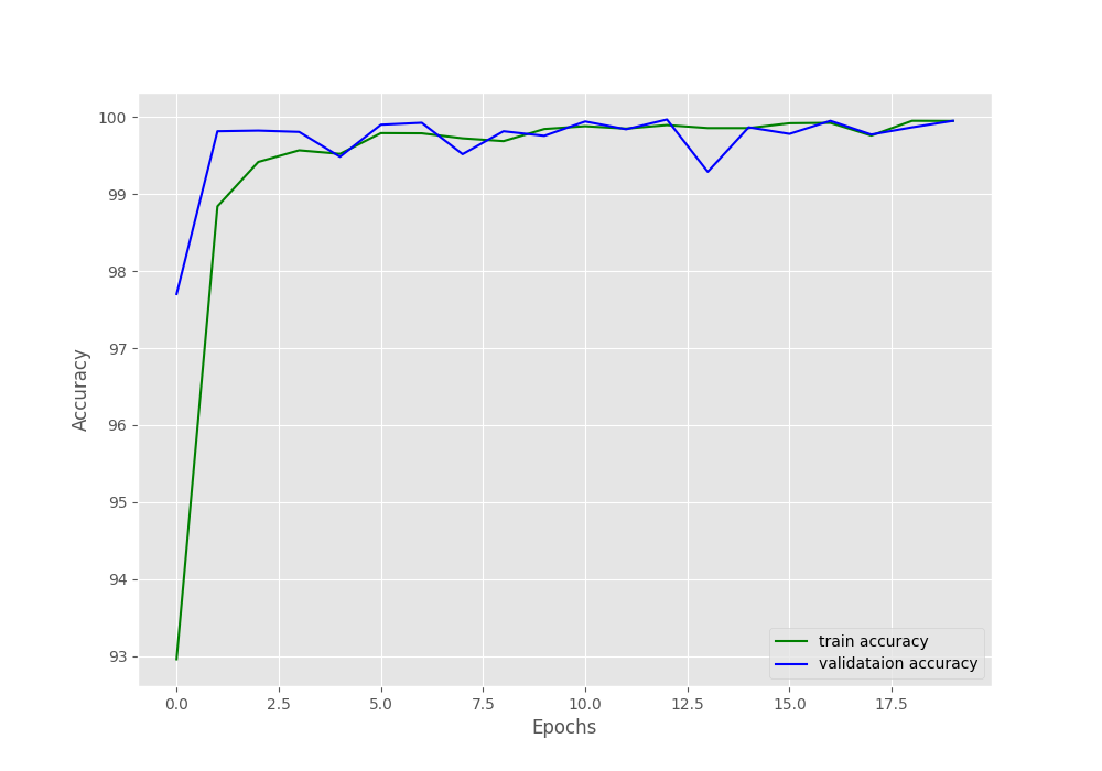
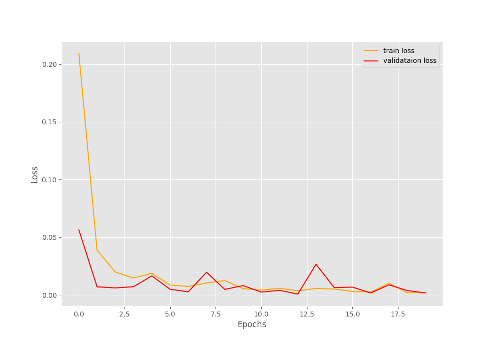
The plots also show minimal fluctuations in the lines. Looks like it is pretty much possible to get 100% validation accuracy with a bit more training by using a learning rate scheduler.

The model is performing really well while training. In the next section, we will write the test script and check out how it performs on the unseen data. We already have the trained model on disk.

Testing the Trained Model on the Unseen Data

Till now, we have trained our PyTorch classifier on the Medical MNIST dataset. The next step is to test it. The test script is going to be completely independent. We could use the functions from the previous utilities. But keeping it independent and writing everything needed in the script is better. It will ensure that anyone who has access to a test set, the trained model, and the test script can easily execute it without any other dependency.

Here, we will accomplish two tasks.

• First one is to calculate the accuracy on the test set.
• The second one is plotting the confusion matrix to check how many instances does the model predict incorrectly.

With that, let’s start writing the code in test.py.

Importing the required modules and setting the constants.

import torch
import torch.nn.functional as F
import numpy as np
import matplotlib.pyplot as plt
import seaborn as sns
import cv2
import torch.nn.functional as F
import torch.nn as nn

from torchvision import transforms, datasets
from torch.utils.data import DataLoader
from tqdm.auto import tqdm
from model import MedicalMNISTCNN
from sklearn.metrics import confusion_matrix

# Constants and other configurations.
TEST_DIR = '../input/medical_mnist_processed/test'
BATCH_SIZE = 1
DEVICE = torch.device('cuda:0' if torch.cuda.is_available() else 'cpu')
IMAGE_RESIZE = 224
NUM_WORKERS = 4
CLASS_NAMES = ['AbdomenCT', 'BreastMRI', 'CXR', 'ChestCT', 'Hand', 'HeadCT']

• We set the test directory path.
• Then the batch size which is 1 in this case. We will iterate over just one sample at a give time which will make it easier for us to carry out other tasks in between the loop.
• Next is the computation device.
• We will resize the images to 224×224 dimensions.
• Number of parallel workers is again 4.
• And then a list containing all the class names. This is for mapping the output class numbers to the actual class names.

The Neural Network Class

We will again define the neural network class here. This might seem repetitive but is quite important to create the standalone test script.

# Define the model architecture.
class MedicalMNISTCNN(nn.Module):
    def __init__(self, num_classes=None):
        super(MedicalMNISTCNN, self).__init__()
        self.conv_block = nn.Sequential(
            nn.Conv2d(in_channels=3, out_channels=32, kernel_size=3),
            nn.ReLU(),
            nn.MaxPool2d(kernel_size=2, stride=2),
            nn.Conv2d(in_channels=32, out_channels=64, kernel_size=3),
            nn.ReLU(),
            nn.MaxPool2d(kernel_size=2, stride=2),
            nn.Conv2d(in_channels=64, out_channels=128, kernel_size=3),
            nn.ReLU(),
            nn.MaxPool2d(kernel_size=2, stride=2),
            nn.Conv2d(in_channels=128, out_channels=256, kernel_size=3),
            nn.ReLU(),
            nn.MaxPool2d(kernel_size=2, stride=2)
        )

        self.classifier = nn.Sequential(
            nn.Linear(in_features=256, out_features=128),
            nn.Dropout2d(p=0.4),
            nn.Linear(in_features=128, out_features=num_classes)
        )

    def forward(self, x):
        x = self.conv_block(x)
        bs, _, _, _ = x.shape
        x = F.adaptive_avg_pool2d(x, 1).reshape(bs, -1)
        x = self.classifier(x)
        return x

Functions to Create Datasets, Data Loader, and Transforms

These are simple functions for creating datasets, iterable loaders, and transforms. They are almost the same as what we did during training.

def test_transform(IMAGE_RESIZE):
    transform = transforms.Compose([
            transforms.Resize((IMAGE_RESIZE, IMAGE_RESIZE)),
            transforms.ToTensor(),
            transforms.Normalize(
                mean=[0.5, 0.5, 0.5],
                std=[0.5, 0.5, 0.5]
                )
        ])
    return transform

def create_test_set():
    dataset_test = datasets.ImageFolder(
        TEST_DIR, 
        transform=(test_transform(IMAGE_RESIZE))
    )
    return dataset_test

def create_test_loader(dataset_test):
    test_loader = DataLoader(
        dataset_test, batch_size=BATCH_SIZE, 
        shuffle=False, num_workers=NUM_WORKERS
    )
    return test_loader

Function to Save Test Image Results

There are more than 5000 images in the test set. We will save a few image predictions to the disk and the following function will help us in doing that.

def save_test_results(tensor, target, output_class, counter):
    """
    This function will save a few test images along with the 
    ground truth label and predicted label annotated on the image.

    :param tensor: The image tensor.
    :param target: The ground truth class number.
    :param output_class: The predicted class number.
    :param counter: The test image number.
    """
    # Move tensor to CPU and denormalize
    image = torch.squeeze(tensor, 0).cpu().numpy()
    image = image / 2 + 0.5
    image = np.transpose(image, (1, 2, 0))
    # Conver to BGR format
    image = cv2.cvtColor(image, cv2.COLOR_RGB2BGR)
    gt = target.cpu().numpy()
    cv2.putText(
        image, f"GT: {CLASS_NAMES[int(gt)]}", 
        (5, 25), cv2.FONT_HERSHEY_SIMPLEX, 
        0.7, (0, 255, 0), 2, cv2.LINE_AA
    )
    cv2.putText(
        image, f"Pred: {CLASS_NAMES[int(output_class)]}", 
        (5, 55), cv2.FONT_HERSHEY_SIMPLEX, 
        0.7, (0, 255, 0), 2, cv2.LINE_AA
    )
    cv2.imwrite(f"../outputs/test_image_{counter}.png", image*255.)

The save_test_results() accepts the image tensor, the target class number, the output class number, and counter (test image number) as parameters.

It first converts the tensor to NumPy array, denormalizes it, and converts into the channels-last format. It also changes the color channels from RGB to BGR as we use OpenCV for annotations and saving the image. All these happen from lines 89 to 93.

After converting the ground-truth to NumPy format, we annotate the test image with the ground-truth label and predicted label. Then we save it to disk by appending the unique counter to the name.

The Test Function

We also need a test function that will iterate through the test data loader and forward pass each image through the model.

def test(model, testloader, DEVICE):
    """
    Function to test the trained model on the test dataset.

    :param model: The trained model.
    :param testloader: The test data loader.
    :param DEVICE: The computation device.

    Returns:
        predictions_list: List containing all the predicted class numbers.
        ground_truth_list: List containing all the ground truth class numbers.
        acc: The test accuracy.
    """
    model.eval()
    print('Testing model')
    predictions_list = []
    ground_truth_list = []
    test_running_correct = 0
    counter = 0
    with torch.no_grad():
        for i, data in tqdm(enumerate(testloader), total=len(testloader)):
            counter += 1
            image, labels = data
            image = image.to(DEVICE)
            labels = labels.to(DEVICE)

            # Forward pass.
            outputs = model(image)
            # Softmax probabilities.
            predictions = F.softmax(outputs).cpu().numpy()
            # Predicted class number.
            output_class = np.argmax(predictions)
            # Append the GT and predictions to the respective lists.
            predictions_list.append(output_class)
            ground_truth_list.append(labels.cpu().numpy())
            # Calculate the accuracy.
            _, preds = torch.max(outputs.data, 1)
            test_running_correct += (preds == labels).sum().item()

            # Save a few test images.
            if counter % 999 == 0:
                save_test_results(image, labels, output_class, counter)

    acc = 100. * (test_running_correct / len(testloader.dataset))
    return predictions_list, ground_truth_list, acc

If you observe, you will notice that we are appending the output class number and the ground truth class number to the predictions_list and ground_truth_list respectively (lines 139 and 140). We return these two lists in the end along with the test accuracy. We need these two lists to plot the confusion matrix.

Also, on line 147, we are saving one test image result after every 999 iterations.

Final Main Block

Let’s combine everything together that will run the testing.

if __name__ == '__main__':
    dataset_test = create_test_set()
    test_loader = create_test_loader(dataset_test)

    checkpoint = torch.load('../outputs/model.pth')
    model = MedicalMNISTCNN(num_classes=6).to(DEVICE)
    model.load_state_dict(checkpoint['model_state_dict'])
    predictions_list, ground_truth_list, acc = test(
        model, test_loader, DEVICE
    )
    print(f"Test accuracy: {acc:.3f}%")
    # Confusion matrix.
    conf_matrix = confusion_matrix(ground_truth_list, predictions_list)
    plt.figure(figsize=(12, 9))
    sns.heatmap(
        conf_matrix, 
        annot=True,
        xticklabels=CLASS_NAMES, 
        yticklabels=CLASS_NAMES
    )
    plt.savefig('../outputs/heatmap.png')
    plt.close()

We create the test dataset and data loader. Then we load the trained model weights and call the test() function. After printing the test set accuracy we get the confusion matrix using Scikit-Learn’s confusion_matrix() function (line 163). Then we plot and save this confusion_matrix (line 165 to 172).

This completes the entire test script. Let’s execute this.

Execute test.py

Execute this script from the same src directory.

python test.py

You should get output similar to the following.

Testing model
100%|█████████████████████████████████████████████████████████████████████████████████████████████████████████████████████████████████████████████████████████████████████████| 5895/5895 [00:08<00:00, 673.03it/s]
Test accuracy: 99.983%

We have 99.983% test accuracy. This is really good. Let’s check out the confusion matrix.

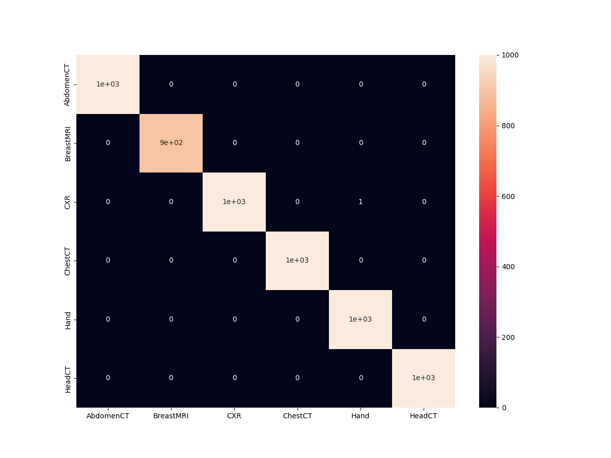
And as expected, the model just made one mistake. It is predicting one Chest X-Ray as Hand.

Finally, let’s take a look at the five test image results saved to disk.

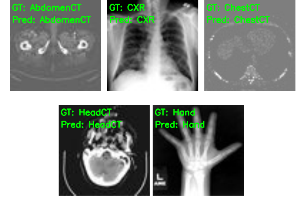
As we already know, the model has predicted these images classes correctly.

Further Steps

As we reach the end of this tutorial, we can conclude that the Medical MNIST dataset is not a particularly difficult dataset to learn for a good enough CNN model. Even our simple model performs really well. Still, there are quite a few things we can improve in this pipeline and experiment further on.

• We can add metrics like precision, recall, f1-score to the pipeline. With other and more complex datasets, this is bound to help.
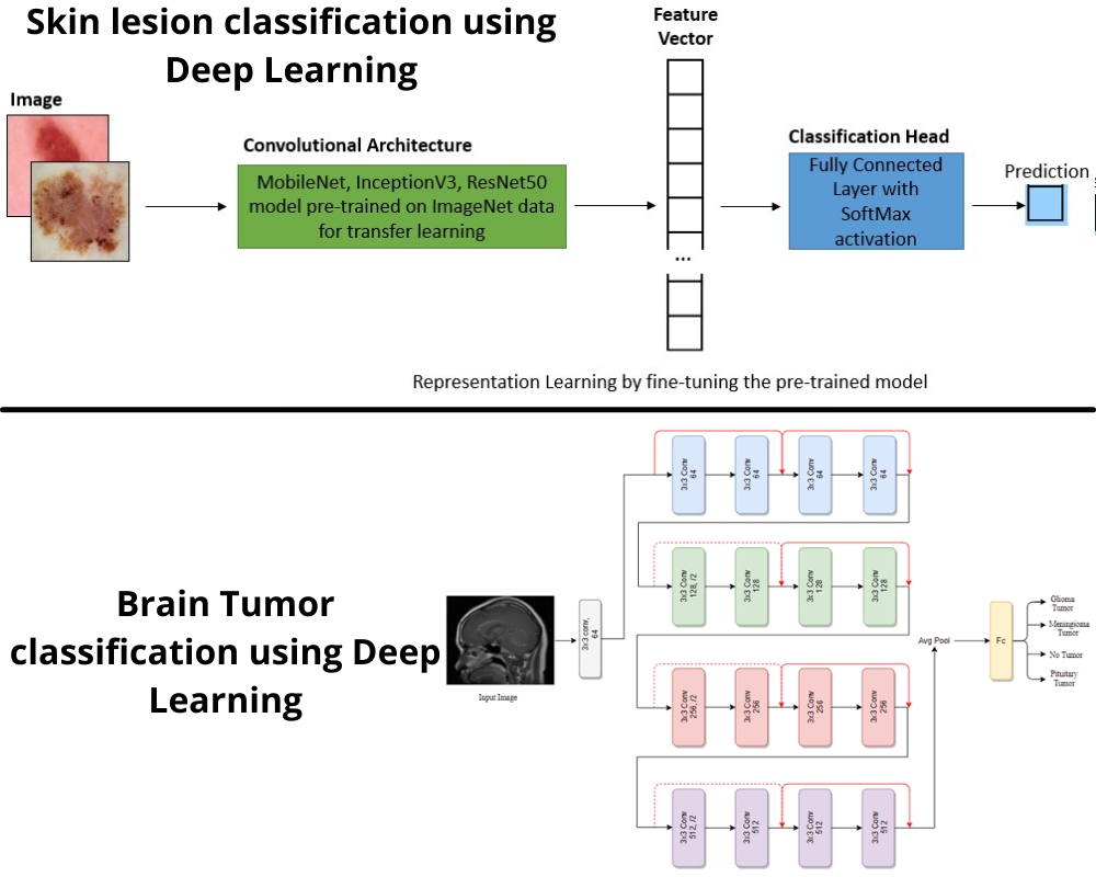
• We now have a trained model which understands a lot of medical imaging features. How about using these features for fine-tuning and classifying on another difficult medical imaging dataset like this one?
• We can also compare our custom PyTorch classifier trained on the Medical MNIST dataset with a pretrained model fine-tuned on the same dataset.

If you carry out any of the above experiments, please let others know in the comment section.

Summary and Conclusion

In this tutorial, we trained a custom PyTorch model on the Medical MNIST dataset. We saw how even a simple model performs really well. We also discussed some further experiments that can be performed regarding the same. I hope that this tutorial was useful to you.

If you have any doubts, thoughts, or suggestions, please leave them in the comment section. I will surely address them.

You can contact me using the Contact section. You can also find me on LinkedIn, and Twitter.