Pneumothorax Binary Classification using PyTorch Model Pretrained on Medical MNIST Dataset

This post is going to be a very interesting one. Here, we will use a custom PyTorch image classification model for Pneumothorax binary classification. Not only that, the model that we will use is not an ImageNet pretrained model. Instead, it is going to be a custom model which has been pretrained on the Medical MNIST dataset.

If you go through the previous post, then you will find that we trained a custom PyTorch image classification model on the Medical MNIST dataset. It gave us a good insight into what CT scans and X-Rays of different body parts look like. Not only that, our model custom model was able to perform pretty well. On the test set, it made only one error. Although the Medical MNIST images were a bit easy to learn for the model. It is fair to say that in the end, we had a model which has learned a lot of features about medical CT scans and X-Ray images.

Pneumothorax is the collapsing of lungs due to a blunt chest injury, damage from underlying lung disease, or it may even occur for no obvious reason at all. At times it can be life-threatening. Being able to identify whether a person has pneumothorax or not can be difficult. But deep learning and computer vision can help here. Training a deep learning model to predict such cases can be a life savior for many. I am not claiming to train a state-of-the-art model in this post. But we will train a reasonably good PyTorch model on the Pneumothorax Binary Classification dataset. Because it is going to be a custom dataset and we will use a few custom metrics, this post will be fun and learning at the same time.

Points to Cover in this Post

In this post, we will take the project from the previous post to the next level. Here, we will take the same custom PyTorch model as the last one along with its pretrained weights. Then we will train the model again on this Pneumothorax Binary Classification dataset from Kaggle. This dataset is considerably more difficult to learn than the Medical MNIST dataset. But hopefully, the pretrained features will help.

Let’s take a look at the points that we will be covering in this post.

• We will start with the exploration of the Pneumothorax Binary Classification dataset from Kaggle.
• Then we will discuss the pretraining of the custom PyTorch model on the Medical MNIST dataset. We will not go into the coding details, instead we will just discuss this part in brief.
• Next, we will moving on to training our custom PyTorch image classification model for Pneumothorax Binary Classification.

I highly recommend going through the previous post where we train a custom PyTorch model on the Medical MNIST dataset. It will give good insights into what we are trying to achieve here.

Further along in this post, we will discuss all the technical and coding details. Hopefully, this will be a good experience for you.

The Pneumothorax Binary Classification Dataset

As discussed earlier, we will use the Pneumothorax Binary Classification dataset for training the PyTorch model. This dataset contains chest x-ray images of lungs. There are 2027 images in this dataset belonging to 2 classes. Either a chest x-ray has Pneumothorax (class 1) or not (class 0).

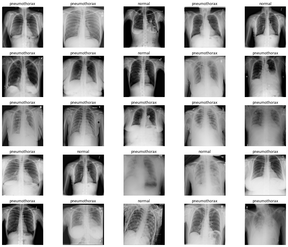
As you can see from the above images, it is not that easy to recognize when a lung has Pneumothorax and when it does not. Hopefully, our deep learning model will do a much better job.

One important thing to note here is that the dataset is highly imbalanced. We have 1597 image samples with Pneumothorax and 430 normal samples. Training a very simple custom model that we have might be very difficult. We will employ a few techniques while training and will take about it further on in the coding section. Also, this post will help us figure out issues with training on such imbalanced datasets and what steps we can take to rectify them.

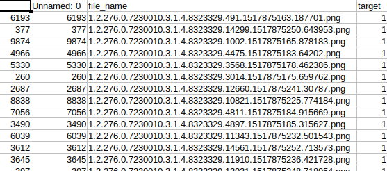
The dataset also contains a CSV file with the image names and the corresponding labels.

The original dataset is part of the SIIM-ACR Pneumothorax Segmentation Kaggle competition. The dataset that we are dealing with in this post has been curated mainly to train image classification models for identifying Pneumothorax in the lungs.

For now, you can download the dataset from here. Later on, we will check how to structure the directory for this project.

Custom PyTorch Model Pretraining on the Medical MNIST Dataset

Here, neither we will train a model from scratch, nor will we use an ImageNet pretrained model. In this post, we will use the same custom model architecture as the previous post and use the weights that have been trained on the Medical MNIST dataset.

We will not go through the pretraining part in this post. Although all the code will be available while downloading the zip file for this post. In case you want to get your hands dirty by carrying out the pretraining yourself, you can do it very easily. The pretraining code is available in the medical_mnist_pretraining.ipynb notebook inside the notebooks directory. You just need to download the Medical MNIST dataset and keep it in the same notebooks directory in the following structure.

medical_mnist
├── AbdomenCT [10000 entries exceeds filelimit, not opening dir]
├── BreastMRI [8954 entries exceeds filelimit, not opening dir]
├── ChestCT [10000 entries exceeds filelimit, not opening dir]
├── CXR [10000 entries exceeds filelimit, not opening dir]
├── Hand [10000 entries exceeds filelimit, not opening dir]
└── HeadCT [10000 entries exceeds filelimit, not opening dir]

But you need not train it on your own if you have computational power constraints as it can take a lot of time. The pretrained model is also provided with the zip file.

The Pretraining Settings and Parameters

We know that we use the same architecture as the previous post. But our pretraining settings differ from the previous post’s training settings in order to have a more robust model.

We have trained the model for 40 epochs using SGD optimizer with an initial learning rate of 0.001. We use Nesterov momentum and weight decay as well. Along with that, we also use the Cosine Annealing Learning Rate Scheduler with warm restarts till the end of 40 epochs. We use 56007 images for training and 2947 images for validation. After the final epoch, we have a validation loss of 0.006 and a validation accuracy of 99.830%.

As the Medical MNIST dataset contains a bit varied images of different CT scans and x-rays, our model might have learned some useful features. This will most probably help in the Pneumothorax Binary Classification with the same PyTorch model.

Directory Structure

Now, let’s take a look at the directory structure for this project.

├── input
│   ├── inference_data
│   │   └── pneumothorax_1.jpg
│   ├── pneumothorax-binary-classification-task
│   │   ├── small_train_data_set
│   │   │   └── small_train_data_set [2028 entries exceeds filelimit, not opening dir]
│   │   └── train_data.csv
│   ├── medical_mnist_pretrained.pth
├── notebooks
│   ├── medical_mnist
│   │   ├── AbdomenCT [10000 entries exceeds filelimit, not opening dir]
│   │   ├── BreastMRI [8954 entries exceeds filelimit, not opening dir]
│   │   ├── ChestCT [10000 entries exceeds filelimit, not opening dir]
│   │   ├── CXR [10000 entries exceeds filelimit, not opening dir]
│   │   ├── Hand [10000 entries exceeds filelimit, not opening dir]
│   │   └── HeadCT [10000 entries exceeds filelimit, not opening dir]
│   ├── eda.ipynb
│   └── medical_mnist_pretraining.ipynb
├── outputs
│   ├── accuracy.png
│   ├── f1_score.png
│   ├── loss.png
│   ├── model.pth
│   ├── normal.png
│   └── pneumothorax.png
├── src
│   ├── datasets.py
│   ├── inference.py
│   ├── model.py
│   ├── train.py
│   └── utils.py

You will get access to a lot of files here when you download the zip file. We will discuss those while going through the directory structure.

• input: This contains two subdirectories, inference_data and pneumothorax-binary-classification-task. inference_data contains the images that we will use for inference after the training is complete. And pneumothorax-binary-classification-task contains the dataset that we get after downloading and extracting the data from Kaggle. If your dataset folder has a different name, you can name it as above for easier training. It also contains a medical_mnist_pretrained.pth file which is the Medical MNIST pretrained model that we will use here.
• notebooks: This contains two notebook, eda.ipynb and medical_mnist_pretraining.ipynb. The EDA notebook contains all the details that we discussed in the dataset exploration section. In case, you may want to train your own model on the Medical MNIST dataset, that you can run the medical_mnist_pretraining.ipynb notebook. You can download the Medical MNIST dataset and put in the structure as in this directory.
• outputs: This will hold the graphs and trained model that training script will generate. This will also hold the image outputs after running inference.
• src: This contains all the Python code files that we need for Pneumothorax binary classification using PyTorch. We will discuss the details while coding through these files.

Except for the datasets, you will get access to all other files when you download the zip file for the tutorial. This includes the trained models as well.

Libraries and Frameworks

There are two major libraries you need for this post. These are PyTorch and Scikit-Learn. The code in this post uses PyTorch 1.10.0 and Scikit-Learn 1.0.1. Please install/upgrade them if you wish to run the code locally.

Pneumothorax Binary Classification using PyTorch

From this section onward, we will start the coding part of this post. We will tackle each Python file in its own subsections. All the code files will remain in the src directory.

Frankly speaking, this project contains quite a lot of code. For that reason, we will not go in-depth into all the general coding stuff. We will surely go through the explanation of those parts which are important.

Let’s get into it then.

Helper Functions

We will need quite a lot of helper functions for training our PyTorch model on the Pneumothorax binary classification dataset. Let’s deal with them first.

All the helper functions will go into the utils.py file.

The first code block contains the import statements and two simple functions.

import torch
import matplotlib
import matplotlib.pyplot as plt
import torch

from sklearn.metrics import f1_score

matplotlib.style.use('ggplot')

def save_model(epochs, model, optimizer, criterion):
    """
    Function to save the trained model to disk.
    """
    torch.save({
                'epoch': epochs,
                'model_state_dict': model.state_dict(),
                'optimizer_state_dict': optimizer.state_dict(),
                'loss': criterion,
                }, f"../outputs/model.pth")

def save_plots(
    train_acc, valid_acc, 
    train_loss, valid_loss,
    train_f1_score, valid_f1_score
):
    """
    Function to save the loss and accuracy plots to disk.
    """
    # Accuracy plots
    plt.figure(figsize=(10, 7))
    plt.plot(
        train_acc, color='green', linestyle='-', 
        label='train accuracy'
    )
    plt.plot(
        valid_acc, color='blue', linestyle='-', 
        label='validataion accuracy'
    )
    plt.xlabel('Epochs')
    plt.ylabel('Accuracy')
    plt.legend()
    plt.savefig(f"../outputs/accuracy.png")
    
    # Loss plots
    plt.figure(figsize=(10, 7))
    plt.plot(
        train_loss, color='orange', linestyle='-', 
        label='train loss'
    )
    plt.plot(
        valid_loss, color='red', linestyle='-', 
        label='validataion loss'
    )
    plt.xlabel('Epochs')
    plt.ylabel('Loss')
    plt.legend()
    plt.savefig(f"../outputs/loss.png")

    # F1 score plots.
    plt.figure(figsize=(10, 7))
    plt.plot(
        train_f1_score, color='purple', linestyle='-', 
        label='train f1 score'
    )
    plt.plot(
        valid_f1_score, color='olive', linestyle='-', 
        label='validataion f1 score'
    )
    plt.xlabel('Epochs')
    plt.ylabel('F1 Score')
    plt.legend()
    plt.savefig(f"../outputs/f1_score.png")

Among the imports, there is f1_score from sklearn as well. We need this to calculate the F1-score while training the model. As you might already be knowing accuracy might not be a very good metric for medical image classification and imbalanced datasets. In such cases, the F1 score works much better as a metric.

And you might also observe that we are plotting the F1-score curves along with loss and accuracy curves in the save_plots() function.

Next, we have three small yet very important functions. The following block contains the code for them.

def get_outputs_binary_list(outputs):
    """
    Function to generate a list of binary values depending on the 
    outputs of the model.
    """
    outputs = torch.sigmoid(outputs)
    binary_list = []
    for i, output in enumerate(outputs):
        if outputs[i] < 0.5:
            binary_list.append(0.)
        elif outputs[i] >= 0.5:
            binary_list.append(1.)
    return binary_list

def binary_accuracy(labels, outputs, train_running_correct):
    """
    Function to calculate the binary accuracy of the model.
    """
    outputs = torch.sigmoid(outputs)
    for i, label in enumerate(labels):
        if label < 0.5 and outputs[i] < 0.5:
            train_running_correct += 1
        elif label >= 0.5 and outputs[i] >= 0.5:
            train_running_correct += 1
    return train_running_correct

def calculate_f1_score(y_true, y_pred):
    """
    Function returns F1-Score for predictions and true labels.
    """
    return f1_score(y_true, y_pred)

The first function is the get_outputs_binary_list(). Our deep learning model will be outputting one logit only as we are solving a binary classification problem. But we need binary output values for calculating the F1-score. This function accepts the logit values for each iteration, passes them through the Sigmoid activation, and appends 1.0 to the binary_list if the Sigmoid value is greater than 0.5. Else, it appends 0.0 to the list.

Next, we have the binary_accuracy() function to calculate the binary accuracy of the deep learning model. This accepts the ground truth labels, the logits (outputs), and the train_running_correct variable to count the number of correct predictions. We return this variable and keep updating it every iteration.

In the end, we have the calculate_f1_score() function which takes the ground truth labels and the predictions which are NumPy arrays. It passes them through the Scikit-Learn’s f1_score and returns the score.

This is all we need for the helper functions.

Preparing the Dataset

Now, we will get on to one of the most important parts of this tutorial. Preparing the Pneumothorax dataset.

The code here will go into the datasets.py Python file.

The first code block contains the imports, a few constants that we need, and reads the CSV file containing the image names and corresponding labels.

import torch
import pandas as pd

from torchvision import transforms
from PIL import Image
from sklearn.model_selection import train_test_split

NUM_WORKERS = 4 # Number of parallel processes for data preparation.
RANDOM_STATE = 42 # To shuffle images and targets in same order.
RESIZE_TO = 256 # Image size to resize to in transforms. 
BATCH_SIZE = 64
ROOT_PATH = '../input/pneumothorax-binary-classification-task'
# Path to images directory.
IMAGES_PATH = f"{ROOT_PATH}/small_train_data_set/small_train_data_set" 

# Load the dataframe.
df = pd.read_csv(f"{ROOT_PATH}/train_data.csv")
# Add extra column with entire image path.
df['image_path'] = IMAGES_PATH + "/" + df.file_name.values

The constants define the:

• Number of workers for the training and validation data loaders.
• The random state that we need while splitting the image paths and labels in training and validation sets.
• Image size to resize to while applying the transforms.
• The batch size with default value of 64. Please reduce it if you face Out Of Memory error while training locally.
• The root path to the dataset and path to the images.

On line 17, we read the CSV file and create an extra image_path column in the data frame which will help us obtain the paths with ease later on.

Functions for Training and Validation Transforms

Next, we are defining functions for applying the training transforms/augmentation and validation transforms as well.

# Training transforms
def get_train_transform(IMAGE_SIZE):
    train_transform = transforms.Compose([
        transforms.Resize((IMAGE_SIZE, IMAGE_SIZE)),
        transforms.RandomCrop(224),
        transforms.RandomAutocontrast(p=0.5),
        transforms.RandomHorizontalFlip(p=0.5),
        transforms.GaussianBlur(kernel_size=(5, 9), sigma=(0.1, 5)),
        transforms.RandomAdjustSharpness(sharpness_factor=2, p=0.5),
        transforms.RandomRotation(45),
        transforms.ToTensor(),
        transforms.Normalize(
            mean=[0.5, 0.5, 0.5],
            std=[0.5, 0.5, 0.5]
            )
    ])
    return train_transform

# Validation transforms
def get_valid_transform(IMAGE_SIZE):
    valid_transform = transforms.Compose([
        transforms.Resize((IMAGE_SIZE, IMAGE_SIZE)),
        transforms.ToTensor(),
        transforms.Normalize(
            mean=[0.5, 0.5, 0.5],
            std=[0.5, 0.5, 0.5]
            )
    ])
    return valid_transform

We are applying quite a lot of augmentations to the training set here. These include:

• Random cropping.
• Applying random contrast.
• Random horizontal flipping.
• Gaussian blurring.
• Random sharpness.
• And random rotation.

Although for medical imaging datasets, it is not always a good idea to apply cropping, as we might lose the region of importance in some cases. We are applying so many augmentations here mainly to compensate for the huge data imbalance.

The get_valid_transform() just resizes the images, converts them to tensors, and normalizes them.

If you observe, you will find that we are applying normalization using mean=[0.5, 0.5, 0.5], std=[0.5, 0.5, 0.5]. If you remember, we will load the Medical MNIST pretrained weights in this post. And that was trained using the same normalizing values. So, it makes sense to apply the same normalization here.

The Dataset Class

We need a Custom PyTorch dataset class for preparing the training and validation sets. It is going to be pretty simple.

class CustomDataset:
    def __init__(self, image_paths, targets, augmentations=None):
        self.image_paths = image_paths
        self.targets = targets
        self.augmentations = augmentations

    def __getitem__(self, idx):
        # Read image.
        image = Image.open(self.image_paths[idx])
        # Convert image to RGB.
        image = image.convert("RGB")
        # Get corresponding target (label).
        targets = self.targets[idx]
        # Apply transforms/augmentations.
        if self.augmentations is not None:
            image = self.augmentations(image)
        # Return images and targets.
        return image, torch.tensor(targets, dtype=torch.float32)

    def __len__(self):
        return len(self.image_paths) 

The image_paths, containing the paths to all images and targets, containing the corresponding labels (either 0 or 1) are lists. augmentation will either hold the train_transform or valid_transform.

We use PIL for reading the image and also convert them to RGB format.

Prepare the Datasets and Data Loaders

Now, it’s time to prepare the training dataset, validation dataset, training data loader, and validation data loader.

# Get all image paths as list
images = df.image_path.values.tolist()
# Get all targets as list.
targets = df.target.values.tolist()

# Split image paths and targets randomly.
train_images, valid_images, train_targets, valid_targets = train_test_split(
    images, targets, test_size=0.20, random_state=RANDOM_STATE
)

# Train dataset and data loader.
def get_datasets():
    train_dataset = CustomDataset(
        image_paths=train_images, 
        targets=train_targets, 
        augmentations=get_train_transform(RESIZE_TO)
    )
    valid_dataset = CustomDataset(
    image_paths=valid_images, 
    targets=valid_targets, 
    augmentations=get_valid_transform(RESIZE_TO)
    )
    return train_dataset, valid_dataset

# Valid dataset and data loader.
def get_data_loaders(train_dataset, valid_dataset):
    train_loader = torch.utils.data.DataLoader(
        train_dataset, 
        batch_size=BATCH_SIZE, 
        shuffle=True, 
        num_workers=NUM_WORKERS
    )
    valid_loader = torch.utils.data.DataLoader(
        valid_dataset, 
        batch_size=BATCH_SIZE, 
        shuffle=False, 
        num_workers=NUM_WORKERS
    )
    return train_loader, valid_loader

On lines 71 and 73, we convert the image paths and labels to a list from the data frame. Then we create the training and validation splits with an 80%-20% ratio respectively.

The get_datasets() function creates the training and validation datasets while applying the respective transforms. And the get_data_loaders() function creates the training and validation data loaders. We will be calling these two functions from the train.py file.

This ends the code for preparing the dataset also.

The Neural Network Model

We will use the same neural network architecture that we used for Medical MNIST classification in the previous post and also for pretraining. It’s a simple network with stackings of convolutional and fully connected layers.

We will write the neural network code in the model.py file.

import torch.nn.functional as F
import torch.nn as nn

class CustomCNN(nn.Module):
    def __init__(self, num_classes=6):
        super(CustomCNN, self).__init__()
        self.conv_block = nn.Sequential(
            nn.Conv2d(in_channels=3, out_channels=32, kernel_size=3),
            nn.ReLU(),
            nn.MaxPool2d(kernel_size=2, stride=2),
            nn.Conv2d(in_channels=32, out_channels=64, kernel_size=3),
            nn.ReLU(),
            nn.MaxPool2d(kernel_size=2, stride=2),
            nn.Conv2d(in_channels=64, out_channels=128, kernel_size=3),
            nn.ReLU(),
            nn.MaxPool2d(kernel_size=2, stride=2),
            nn.Conv2d(in_channels=128, out_channels=256, kernel_size=3),
            nn.ReLU(),
            nn.MaxPool2d(kernel_size=2, stride=2)
        )

        self.classifier = nn.Sequential(
            nn.Linear(in_features=256, out_features=128),
            nn.Dropout2d(p=0.4),
            nn.Linear(in_features=128, out_features=num_classes)
        )

    def forward(self, x):
        x = self.conv_block(x)
        bs, _, _, _ = x.shape
        x = F.adaptive_avg_pool2d(x, 1).reshape(bs, -1)
        x = self.classifier(x)
        return x

You can see the num_classes parameter has a default value of 6. We will use this default value for initializing the model as the Medical MNIST dataset had 6 classes. So, the pretrained weights will be expecting 6 classes in the final layer. We will change that after loading the weights.

There is not much to explain in this architecture as it is a very simple image classification model.

The Training Script

We need to write the code for the training script before we can begin the training. It is going to be a bit big but most of the things will be simple. There are a few important things which we will go through for sure.

All the code for the training script will be in the train.py file.

The following code block contains the import statements and the construction of the argument parser.

import torch
import argparse
import torch.nn as nn
import torch.optim as optim

from tqdm.auto import tqdm

from model import CustomCNN
from datasets import (
    get_datasets, get_data_loaders
)
from utils import (
    save_model, save_plots,
    get_outputs_binary_list, 
    binary_accuracy, calculate_f1_score
)
# Construct the argument parser.
parser = argparse.ArgumentParser()
parser.add_argument(
    '-e', '--epochs', type=int, default=10,
    help='Number of epochs to train our network for'
)
parser.add_argument(
    '-lr', '--learning-rate', type=float,
    dest='learning_rate', default=0.001,
    help='Learning rate for training the model'
)
args = vars(parser.parse_args())

We are importing every module whose functions we need to call from here. And we control the number of epochs to train for and the learning rate from the command line using --epochs and --learning-rate flags respectively.

The Training Function

The training function is going to be a bit different in this post. We need to calculate the binary accuracy and the F1-score. Along with that, we will use a weight tensor for the classes for proper loss weightage as we have a class imbalance issue here.

# Training function.
def train(model, trainloader, optimizer, criterion, scheduler=None, epoch=None):
    model.train()
    print('Training')
    train_running_loss = 0.0
    train_running_correct = 0
    counter = 0
    y_true = []
    y_pred = [] 
    iters = len(trainloader)
    for i, data in tqdm(enumerate(trainloader), total=len(trainloader)):
        counter += 1
        image, labels = data
        image = image.to(device)
        labels = labels.to(device)
        optimizer.zero_grad()
        # Forward pass.
        outputs = model(image)

        # Calculate the loss.
        loss = criterion(outputs, labels.view(-1, 1))
        train_running_loss += loss.item()

        # Get the binary predictions, 0 or 1.
        outputs_binary_list = get_outputs_binary_list(
            outputs.clone().detach().cpu()
        )
        # Calculate the accuracy.
        train_running_correct = binary_accuracy(
            labels, outputs, train_running_correct
        )
        # Backpropagation.
        loss.backward()
        # Update the weights.
        optimizer.step()

        if scheduler is not None:
            scheduler.step(epoch + i / iters)
        y_true.extend(labels.detach().cpu().numpy())
        y_pred.extend(outputs_binary_list)
        
    # Loss and accuracy for the complete epoch.
    epoch_loss = train_running_loss / counter
    epoch_acc = 100. * (train_running_correct / len(trainloader.dataset))
    # F1 score.
    f1_score = calculate_f1_score(y_true, y_pred)
    return epoch_loss, epoch_acc, f1_score

First, let’s take a look at all the variables.

• train_running_loss: To keep adding the loss of each batch for an entire epoch.
• train_running_correct: To keep adding the accuracy of each batch.
• y_true: For storing the ground truth values of each batch.
• y_pred: For storing the predicted labels of each batch.

After calculating the loss on line 49, we add it to the train_running_loss. Then we get the binary outputs on line 53, count the number of correct predictions on line 57, do the backward pass, and update the model weights. If we pass any scheduler, then its step incrementation happens on line 66. Just as a heads up, we will use the Cosine Annealing with Warm Restarts scheduler while training. We then append the ground truths and predictions to the respective lists.

We calculate the loss, binary accuracy, and F1-score for the epoch and return these.

The Validation Function

In the validation function, we return the loss, accuracy, and F1-score just as we do in the training function. But we do not need any backpropagation here.

# Validation function.
def validate(model, testloader, criterion):
    model.eval()
    print('Validation')
    valid_running_loss = 0.0
    valid_running_correct = 0
    y_true = []
    y_pred = []
    counter = 0
    with torch.no_grad():
        for i, data in tqdm(enumerate(testloader), total=len(testloader)):
            counter += 1
            
            image, labels = data
            image = image.to(device)
            labels = labels.to(device)
            # Forward pass.
            outputs = model(image)

            # Calculate the loss.
            loss = criterion(outputs, labels.view(-1, 1))
            valid_running_loss += loss.item()

            # Get the binary predictions, 0 or 1.
            outputs_binary_list = get_outputs_binary_list(
                outputs.clone().detach().cpu()
            )
            # Calculate the accuracy.
            valid_running_correct = binary_accuracy(
                labels, outputs, valid_running_correct
            )
            y_true.extend(labels.detach().cpu().numpy())
            y_pred.extend(outputs_binary_list)
        
    # Loss and accuracy for the complete epoch.
    epoch_loss = valid_running_loss / counter
    epoch_acc = 100. * (valid_running_correct / len(testloader.dataset))
    # F1 score.
    f1_score = calculate_f1_score(y_true, y_pred)
    return epoch_loss, epoch_acc, f1_score

The Main Code Block

The main code block will encapsulate everything that we did in the training script till now and also connect all the elements of the previous module.

if __name__ == '__main__':
    # Load the training and validation datasets.
    train_dataset, valid_dataset = get_datasets()
    # Load the training and validation data loaders.
    train_loader, valid_loader = get_data_loaders(
        train_dataset, valid_dataset
    )
    print(f"[INFO]: Number of training images: {len(train_dataset)}")
    print(f"[INFO]: Number of validation images: {len(valid_dataset)}")

    # Learning_parameters. 
    lr = args['learning_rate']
    epochs = args['epochs']
    device = ('cuda' if torch.cuda.is_available() else 'cpu')
    print(f"Computation device: {device}")
    print(f"Learning rate: {lr}")
    print(f"Epochs to train for: {epochs}\n")

    model = CustomCNN()
    checkpoint = torch.load('../input/medical_mnist_pretrained.pth', map_location='cuda')
    model.load_state_dict(checkpoint['model_state_dict'])
    model.classifier[2] = nn.Linear(in_features=128, out_features=1)
    model = model.to(device)
    
    # Total parameters and trainable parameters.
    total_params = sum(p.numel() for p in model.parameters())
    print(f"{total_params:,} total parameters.")
    total_trainable_params = sum(
        p.numel() for p in model.parameters() if p.requires_grad)
    print(f"{total_trainable_params:,} training parameters.")

    # Optimizer.
    optimizer = optim.AdamW(model.parameters(), lr=lr)
    # Loss function.
    criterion = nn.BCEWithLogitsLoss()

    scheduler = torch.optim.lr_scheduler.CosineAnnealingWarmRestarts(
        optimizer, 
        T_0=25, 
        T_mult=1,
        verbose=True
    )

    # Lists to keep track of losses and accuracies.
    train_loss, valid_loss = [], []
    train_acc, valid_acc = [], []
    train_f1_score, valid_f1_score = [], []
    # Start the training.
    for epoch in range(epochs):
        print(f"[INFO]: Epoch {epoch+1} of {epochs}")
        train_epoch_loss, train_epoch_acc, train_epoch_f1_score = train(
            model, train_loader, 
            optimizer, criterion,
            scheduler=scheduler, epoch=epoch
        )
        valid_epoch_loss, valid_epoch_acc, valid_epoch_f1_score = validate(
            model, valid_loader,  criterion
        )
        train_loss.append(train_epoch_loss)
        valid_loss.append(valid_epoch_loss)
        train_acc.append(train_epoch_acc)
        valid_acc.append(valid_epoch_acc)
        train_f1_score.append(train_epoch_f1_score)
        valid_f1_score.append(valid_epoch_f1_score)
        print(
            f"Training loss: {train_epoch_loss:.3f},",
            f"training acc: {train_epoch_acc:.3f},",
            f"training f1-score: {train_epoch_f1_score:.3f}"
            )
        print(
            f"Validation loss: {valid_epoch_loss:.3f},",
            f"validation acc: {valid_epoch_acc:.3f},",
            f"validation f1-score: {valid_epoch_f1_score:.3f}"
            )
        print(f"LR at end of epoch {epoch+1} {scheduler.get_last_lr()[0]}")
        print('-'*50)
        
    # Save the trained model weights.
    save_model(epochs, model, optimizer, criterion)
    # Save the loss and accuracy plots.
    save_plots(
        train_acc, valid_acc, 
        train_loss, valid_loss, 
        train_f1_score, valid_f1_score
    )
    print('TRAINING COMPLETE')

The following points cover everything that the if name == 'main' block does:

• We start with preparing the datasets and data loaders.
• Then we define the learning parameters like the learning rate and the number of epochs along with the computation device.
• The important things happen from line 134 to line 138. First, we initialize the CustomCNN() architecture. At this point, the last classification layer contains 6 output units. Then we load the Medical MNIST pretrained weights into the model. On line 137, we change the number of output units to 1 as we are solving a binary classification problem here and move the model to the computation device.
• On lines 148 and 150, we define the optimizer and Binary Cross Entropy loss function. As the last layer of the network does not contain the sigmoid activation function, we use the BCEWithLogitsLoss.
• Then we define the CosineAnnealingWarmRestarts scheduler where the learning rate will restart every 25 epochs.
• From lines 160 to 162 we define lists to store losses, accuracies, and F1-scores.
• Line 164 starts the training loop.
• Note that we pass the scheduler to the train function. If you don’t intend to apply the scheduler for any experiments, simply pass None.
• After every epoch, we print the information on the screen.
• At the end of the training, we save the model and the accuracy, loss, and F1-score plots to the disk.

With this, we finish all the code that we need to train our PyTorch model on the Pneumothorax binary image classification dataset.

Execute train.py to Start the Training

To start the training, open the command line/terminal in the src directory and execute the following command.

python train.py --epochs 100 --learning-rate 0.0001

We train for 100 epochs with a learning rate of 0.0001. The learning rate will become 0 every 25 epochs and again restart.

The following block contains the truncated output.

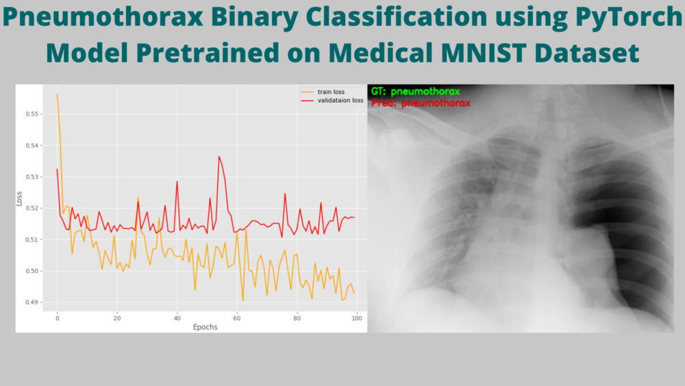
[INFO]: Number of training images: 1621
[INFO]: Number of validation images: 406
Computation device: cuda
Learning rate: 0.0001
Epochs to train for: 100

421,441 total parameters.
421,441 training parameters.
Epoch     0: adjusting learning rate of group 0 to 1.0000e-04.
[INFO]: Epoch 1 of 100
Training
100%|██████████████████████████████████████████████████████████████████████████████████████████████████████████████████████████████████████████████████████████████████████████████| 26/26 [00:05<00:00,  4.54it/s]
Validation
100%|████████████████████████████████████████████████████████████████████████████████████████████████████████████████████████████████████████████████████████████████████████████████| 7/7 [00:01<00:00,  5.26it/s]
Training loss: 0.556, training acc: 77.051, training f1-score: 0.869
Validation loss: 0.532, validation acc: 77.340, validation f1-score: 0.870
LR at end of epoch 1 9.96354437049027e-05
--------------------------------------------------
[INFO]: Epoch 2 of 100
Training
100%|██████████████████████████████████████████████████████████████████████████████████████████████████████████████████████████████████████████████████████████████████████████████| 26/26 [00:05<00:00,  4.56it/s]
Validation
100%|████████████████████████████████████████████████████████████████████████████████████████████████████████████████████████████████████████████████████████████████████████████████| 7/7 [00:01<00:00,  5.25it/s]
Training loss: 0.543, training acc: 78.347, training f1-score: 0.877
Validation loss: 0.518, validation acc: 76.847, validation f1-score: 0.869
LR at end of epoch 2 9.848869081092581e-05
--------------------------------------------------
...
[INFO]: Epoch 99 of 100
Training
100%|██████████████████████████████████████████████████████████████████████████████████████████████████████████████████████████████████████████████████████████████████████████████| 26/26 [00:05<00:00,  4.52it/s]
Validation
100%|████████████████████████████████████████████████████████████████████████████████████████████████████████████████████████████████████████████████████████████████████████████████| 7/7 [00:01<00:00,  5.32it/s]
Training loss: 0.496, training acc: 79.272, training f1-score: 0.884
Validation loss: 0.517, validation acc: 76.847, validation f1-score: 0.869
LR at end of epoch 99 4.251323616870029e-07
--------------------------------------------------
[INFO]: Epoch 100 of 100
Training
100%|██████████████████████████████████████████████████████████████████████████████████████████████████████████████████████████████████████████████████████████████████████████████| 26/26 [00:05<00:00,  4.53it/s]
Validation
100%|████████████████████████████████████████████████████████████████████████████████████████████████████████████████████████████████████████████████████████████████████████████████| 7/7 [00:01<00:00,  5.21it/s]
Training loss: 0.493, training acc: 79.087, training f1-score: 0.883
Validation loss: 0.517, validation acc: 76.847, validation f1-score: 0.869
LR at end of epoch 100 5.839991235656595e-10
--------------------------------------------------
TRAINING COMPLETE

Looking at the graphs will give us more insights.

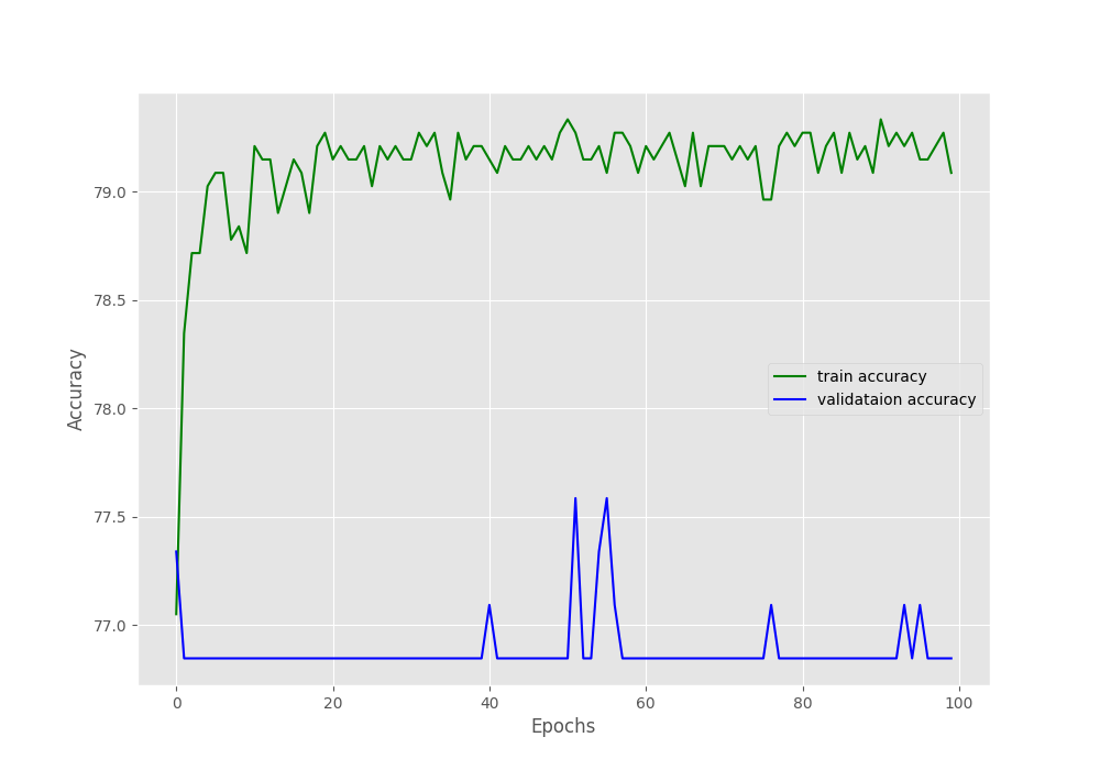
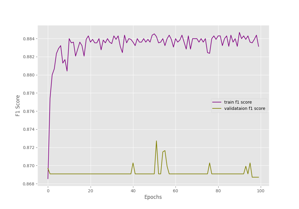
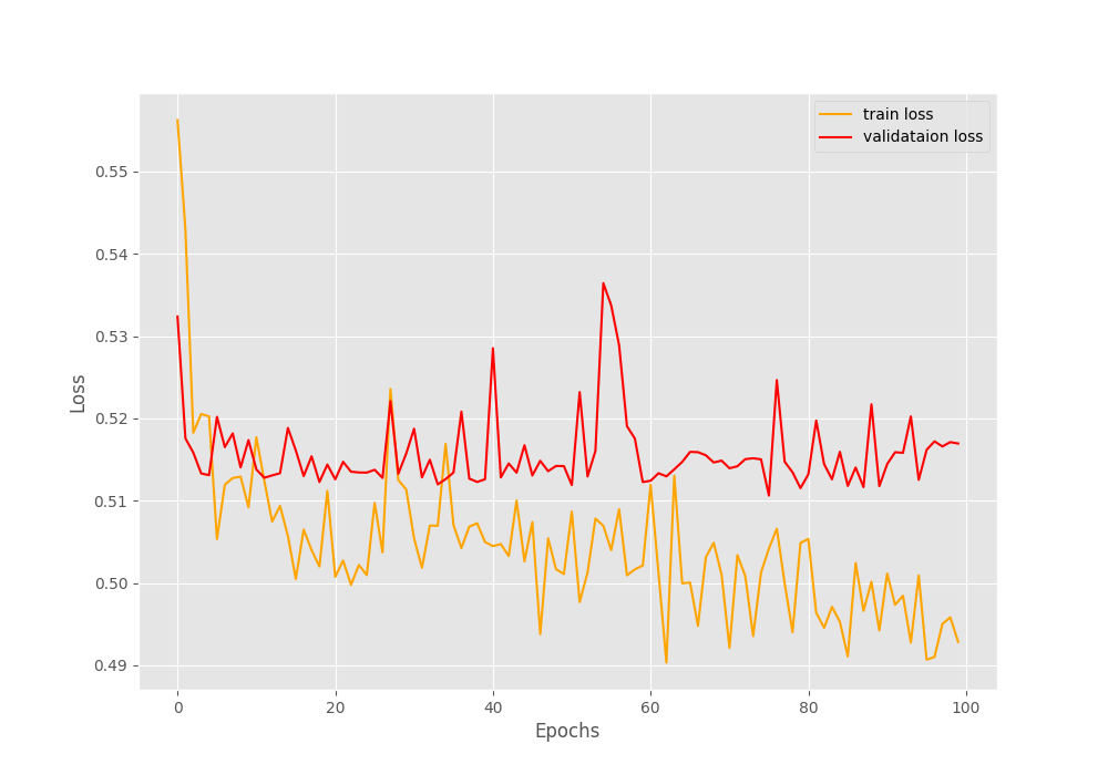
Okay! so, what is happening here?

Starting with the accuracy graphs, we can clearly see that the training plot is increasing till the end of training. But the validation accuracy is flattened at around 77.8% after the first epoch.

The F1-score also follows a similar trend.

The only indication that we have the model might be learning is from the loss graphs. The training loss is decreasing but the validation loss seems not to improve.

What could be the reason for such results?

Remember that, in our dataset around 1600 images have Pneumothorax and around 400 images have negative classes (normal lung x-rays). This is highly skewed for sure. And the validation set might be containing mostly positive class images which lead to the plateauing of the accuracy and F1-score.

We can infer that this is a big issue and the model might only learn the features of Pneumothorax lung x-rays and overfit on that. This may affect the inference on new and unseen images. But we can only conclude that once we carry out the inference.

Inference Using the Trained Model

This is the final coding section in this post. Here, we will write the script to carry out inference on a few inference images that are downloaded from the internet.

The inference code will go into the inference.py script.

Starting with importing the modules, defining the constants, loading the trained model, and defining the transforms.

import torch
import cv2
import glob as glob
import os

from model import CustomCNN
from torchvision import transforms

# Constants.
DATA_PATH = '../input/inference_data'
IMAGE_SIZE = 224
DEVICE = 'cpu'

# Load the trained model.
model = CustomCNN(num_classes=1)
checkpoint = torch.load('../outputs/model.pth', map_location=DEVICE)
print('Loading trained model weights...')
model.load_state_dict(checkpoint['model_state_dict'])

transform = transforms.Compose([
        transforms.ToPILImage(),
        transforms.Resize((IMAGE_SIZE, IMAGE_SIZE)),
        transforms.ToTensor(),
        transforms.Normalize(
            mean=[0.5, 0.5, 0.5],
            std=[0.5, 0.5, 0.5]
        )
    ]) 

After the imports, the constants contain the inference image paths, image resize value and the computation device. Then we load the model weights and define the preprocessing transforms.

Next is capturing all the image paths and looping over them while carrying out inference on each image.

# Get all the test image paths.
all_image_paths = glob.glob(f"{DATA_PATH}/*")

# Iterate over all the images and do forward pass.
for image_path in all_image_paths:
    # Get the ground truth class name from the image path.
    gt_class_name = image_path.split(
        os.path.sep
    )[-1].split('.')[0].split('_')[0]
    # Read the image and create a copy.
    image = cv2.imread(image_path)
    orig_image = image.copy()
    
    # Preprocess the image.
    image = cv2.cvtColor(image, cv2.COLOR_BGR2RGB)
    image = transform(image)
    image = torch.unsqueeze(image, 0)
    image = image.to(DEVICE)
    
    # Forward pass throught the image.
    outputs = model(image)
    output_sigmoid = torch.sigmoid(outputs)
    pred_class_name = 'pneumothorax' if output_sigmoid > 0.5 else 'normal'
    print(f"GT: {gt_class_name}, Pred: {pred_class_name.lower()}")
    # Annotate the image with ground truth.
    cv2.putText(
        orig_image, f"GT: {gt_class_name}",
        (10, 25), cv2.FONT_HERSHEY_SIMPLEX,
        0.8, (0, 255, 0), 2, lineType=cv2.LINE_AA
    )
    # Annotate the image with prediction.
    cv2.putText(
        orig_image, f"Pred: {pred_class_name.lower()}",
        (10, 55), cv2.FONT_HERSHEY_SIMPLEX,
        0.8, (0, 0, 225), 2, lineType=cv2.LINE_AA
    ) 
    cv2.imshow('Result', orig_image)
    print(gt_class_name)
    cv2.waitKey(0)
    cv2.imwrite(
        f"../outputs/{image_path.split(os.path.sep)[-1].split('.')[0]}.png",
        orig_image
    )

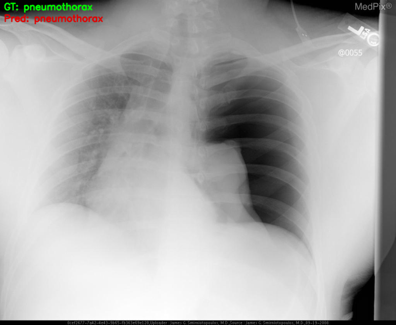
After the forward pass, we obtain the prediction class name according to the sigmoid outputs (line 51). Then print the outputs, annotate the ground truth and prediction label on the image, visualize them and save them to disk.

Let’s execute the inference.py script from the same src directory and check out the predictions.

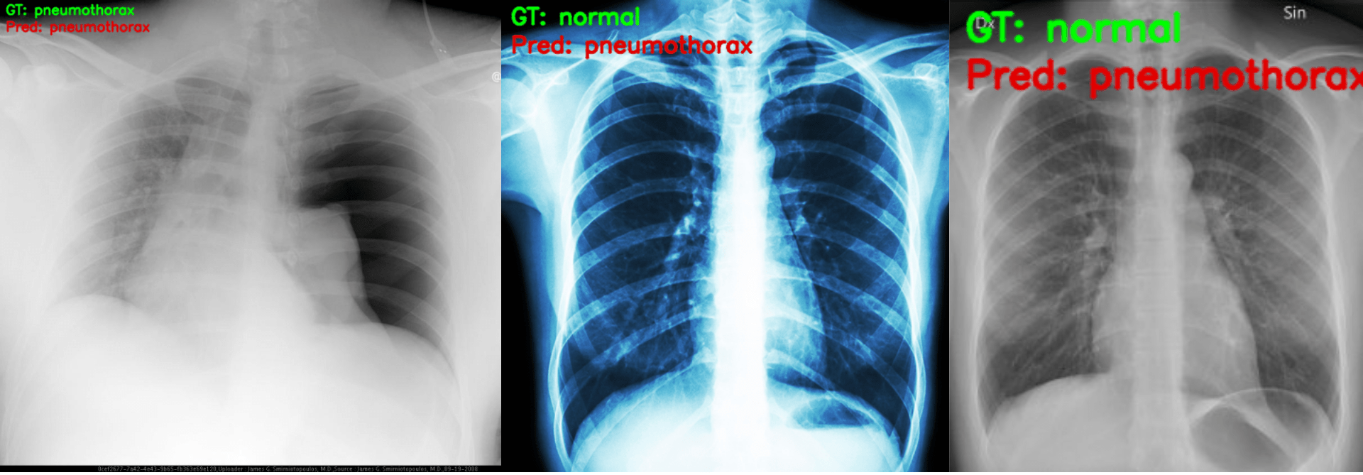
python inference.py 

The outputs on the terminal.

Loading trained model weights...
GT: pneumothorax, Pred: pneumothorax
GT: normal, Pred: pneumothorax
GT: normal, Pred: pneumothorax

We can already see that only one prediction is correct. The model is predicting all images as pneumothorax just as we had anticipated it might.

Analysis and Further Steps

The results that we obtained in this post are surely the because of not having enough negative classes. Our model was not able to learn properly what a normal lung x-ray looks like.

So, how to overcome this?

• One of the easiest steps that we can take is applying oversampling to the negative classes. We can apply augmentations to the images and save to disk before hand. This will ensure that we can have roughly the same number of positive and negative classes while training.
• Another way is to apply a large set of augmentations dynamically to the negative samples when the dataset is prepared. Although this approach is not guranteed to help, still worth a try.

In the next post, we will try the oversampling of the negative classes approach and see how the model performs. So, stay tuned for that.

Summary and Conclusion

In this post, we tried binary image classification on a Pneumothorax dataset using a custom PyTorch model which was pretrained on the Medical MNIST dataset. We got to know the issues that one faces when trying to deal with imbalanced dataset with very less number of negative classes. We will try to solve this issue in the next post. I hope that this post was helpful to you.

If you have any doubts, thoughts, or suggestions, please leave them in the comment section. I will surely address them.

You can contact me using the Contact section. You can also find me on LinkedIn, and Twitter.

Credits for Images Used for Inference

• pneumothorax_1.jpg: https://medpix.nlm.nih.gov/search?allen=true&allt=true&alli=true&query=pneumothorax.
• normal_1.jpg: https://glassboxmedicine.com/2019/02/10/radiology-normal-chest-x-rays/.
• normal_2.png: https://kinkaidprivatecare.com/normal-chest-x-ray/.