PyTorch Implementation of Stochastic Gradient Descent with Warm Restarts

In this tutorial, we are going to carry out PyTorch implementation of Stochastic Gradient Descent with Warm Restarts. In the previous article , we learned about Stochastic Gradient Descent with Warm Restarts along with the details in the paper. This article is going to be completely practical.

We will try to replicate a small part of the experiment of the paper. We will use the PyTorch deep learning framework to implement the paper. So, further in this article, we will carry out PyTorch implementation of Stochastic Gradient Descent with Warm Restarts.

Before, moving further, let’s see what we will be covering in this tutorial?

• An overview of the hyperparameters and training parameters from the original SGDR paper.
• What changes will we be making to make the paper implementation a bit more feasible?
• Coding our way through PyTorch implementation of Stochastic Gradient Descent with Warm Restarts.
• Analyzing and comparing results with that of the paper.

I hope that you are excited to follow along with me till the end. And yes, if you are new to the topic of Stochastic Gradient Descent with Warm Restarts, then you may find this previous article really helpful. In specific, you will find details about the following in the previous post:

• What is Stochastic Gradient Descent with Warm Restarts in Deep Learning?
• How Warm Restarts are used for learning rate scheduling?
• Cosine Annealing for the learning rate update in each batch?
• Details about the experiments and results done by the authors of the paper.
• What are the advantages of Stochastic Gradient Descent with Warm Restarts?

If you are completely new to the topic, then you will find the article useful.

Now, let’s move forward with the implementation of the SGDR.

Training and Experiment Setup

In this section, we will go through the training and experiment setup that we will use for the PyTorch implementation of the paper.

First, we will go through the hyperparameter settings that the authors used for their experiments. We will make a few changes to that which we will go through as well. After that, we will be all set to start our coding part.

Hyperparameter and Training Settings in the Original SGDR Paper

The authors (Ilya Loshchilov & Frank Hutter) have explained quite well what were the hyperparameter and training settings in their experiments. They have also mentioned the particular neural network model as well. The following are the hyperparameter settings:

• First of all, the authors needed to compare their results with something to get a benchmark. So, the baseline they used was with a default learning rate schedule. This scheduling technique was proposed in the Wide Residual Networks paper by Zagoruyko & Komodakis (2016). As per this, the default learning rate schedule is changing the learning rates at epochs 60, 120, and 160 by a factor of 0.2
• The authors use the SGD optimizer with a starting learning rate of 0.05, weight decay of 0.0005, set the dampening to 0, and momentum to 0.9.
• For the datasets, they use CIFAR-10 and CIFAR-100 with a minibatch of 128. They use horizontal flipping and random cropping for image augmentations.
• For the neural network model, they choose Wide Residual Network (WRN). They carry out experiments with both WRN-28-10 and WRN-28-20. If you wish to know more about WRNs, then you can find more details in the original paper. They trained the model for 200 epochs.
• The authors also ran experiments for ensemble models and multiple times as well to get the results at different ensemble snapshots.

That is quite a big list. We will follow most of the procedure, except a few changes. We will cover that next.

Hyperparameter and Training Settings that We will Use

We will keep most of the settings the same as above. But we will have to make a few changes to keep the implementation simple and the training short as well.

• First of all, we will not use Wide Residual Networks. Wide Residual Networks have quite a large number of parameters, in the range of 36 million. And training for 200 epochs can take a long time to complete. Instead, we will the ResNet34 deep learning model. That model is just the right size to carry out this PyTorch experiment.
• Next, we will also skip the model ensembling experiments for obvious reasons. The amount of computing power that we will need for completing all the runs is just too large. So, we will skip it.
• Also, we will carry our PyTorch implementation of SGDR on just the CIFAR-10 dataset and not the CIFAR-100. The reason again being the training time and computing power required.

So, the above are all the changes that we will make. Still, if you want, you can go through Section 4.1 of the SGDR paper to get the hyperparameter details.

As of now, we are all set to start our PyTorch experimentation. Before starting to code, there is just one thing left.

Directory Structure and PyTorch Version

We will keep a simple and easy to follow directory structure. The following block shows the project directory structure.

│   models.py
│   plot.py
│   run.sh
│   train.py
│
├───data
│   │   cifar-10-python.tar.gz
│
├───outputs

• Directly inside the project directory, we have three Python code files and one shell script. We will get into the details of these while writing the code.
• The data folder contains the CIFAR-10 dataset that will download using torchvision.datasets.
• And finally, the outputs folder will contain all the output files and plots that will be generated while training and validation.

As for the PyTorch version, I have used PyTorch 1.7.1, which is the latest at the time of this writing. You should not be facing any issues if you have slightly older version. But still, it will be better if you can use the latest version as well.

Now, we are all set to start coding and implement the SGDR paper using PyTorch.

PyTorch Implementation of Stochastic Gradient Descent with Warm Restarts – The Coding Part

Though a very small experiment of the original SGDR paper, still, this should give us a pretty good idea of what to expect when using cosine annealing with warm restarts to train deep neural networks.

Now, we have three Python files and we will start with the preparation of our ResNet34 neural network archtitecture.

The PyTorch ResNet34 Model

It is going to be simple. We will use the models module from torchvision to prepare the ResNet34 neural network architecture. And all the code in this section will go into the models.py Python file.

Before going further, there are few things to keep in mind.

• The authors did not use a pre-trained Wide ResNet for training. We are using ResNet34 and we will not be using a pre-trained model.
• Along with that, all the intermediate layers’ parameters will be trainable. Just as in the case of the research paper.

The following code block defines the ResNet34 deep learning model that we will use.

from torchvision import models as models
import torch.nn as nn

def resnet34(pretrained, requires_grad):
    model = models.resnet34(progress=True, pretrained=pretrained)
    # to freeze the hidden layers
    if requires_grad == False:
        for param in model.parameters():
            param.requires_grad = False
    # to train the hidden layers
    elif requires_grad == True:
        for param in model.parameters():
            param.requires_grad = True
    # make the classification layer learnable
    # we have 10 classes in total for the CIFAR10 dataset
    model.fc = nn.Linear(512, 10)
    return model

• We will pass the pretrained and requires_grad arguments as per our requirement, that is, False and True respectively.
• We are also changing the output features in the last layer to 10 to match the number of classes to that of CFIAR-10.

This is all the code we need to prepare the model.

Python Code for Training the Neural Network

In this section, we will write the training code. This training code will go into the train.py file.

The following are all the modules and libraries that we need along the way for the training code.

import torch
import torchvision
import torchvision.transforms as transforms
import matplotlib.pyplot as plt
import matplotlib
import torch.nn as nn
import torch.optim as optim
import models
import argparse
import joblib

from tqdm import tqdm

matplotlib.style.use('ggplot')

Along with all the standard imports, we are also importing our own models module.

Next, we will define the argument parser and the computation device.

parser = argparse.ArgumentParser()
parser.add_argument('-wr', '--warm-restart', dest='warm_restart', 
                    action='store_true')
parser.add_argument('-t0', '--t-zero', dest='t_zero', type=int,
                    default=50)
parser.add_argument('-tm', '--t-mult', dest='t_mult', type=int,
                    default=1)
parser.add_argument('-e', '--epochs', type=int, default=100)
args = vars(parser.parse_args())

device = torch.device('cuda' if torch.cuda.is_available() else 'cpu')
print(f"[INFO]: Computation device: {device}")
epochs = args['epochs']
batch_size = 128 # same the original paper

Going over the flags for the argument paser:

• --warm-restart: Passing this argument while training will ensure that Cosine Annealing with Warm Restarts is used while training.
• --t-zero: This flag defines the initial number of epochs for the first warm restart. This is the same \(T_0\) as the paper.
• --t-mult: This flag is the multiplicative factor for the number of epochs for the warm restart. It is the \(T_{mult}\) argument from the paper.
• --epochs: It is simply the number of epochs that we want to train for.

After that, we also define the computation device at line 25. Line 26 stores the number of epochs in the epochs variable. And for the batch size, we will be using the exact same number as the paper, which is 128.

The Image Augmentations and Preparing the Dataset

In this part, we will define the training and validation transforms and augmentations for the CIFAR-10 dataset. We will follow the same augmentations for training as in the paper (Details in Section 4.1).

# we will apply the same transforms as described in the paper
train_transform = transforms.Compose(
    [transforms.RandomHorizontalFlip(),
     transforms.RandomCrop(size=(32, 32), padding=4, padding_mode='reflect'),
     transforms.ToTensor(),
     transforms.Normalize((0.4914, 0.4822, 0.4465), (0.247, 0.243, 0.261))])
val_transform = transforms.Compose(
    [transforms.ToTensor(),
     transforms.Normalize((0.4914, 0.4822, 0.4465), (0.247, 0.243, 0.261))])

Let’s go over the training transforms and augmentations:

• We are using RandomHorizontalFlip() which was also done for the research paper experiments.
• The random cropping is also according to the paper. We are padding by 4 pixels on each side and filling any missing data using mirror reflections of the image.
• After converting the pixels to tensors, we are normalizing them using the CIFAR-10 stats.

For the validation transforms, we are only converting the pixels to tensors and normalizing them.

Next, we have the datasets and the data loaders.

train_dataset = torchvision.datasets.CIFAR10(root='./data', train=True,
                                             download=True, 
                                             transform=train_transform)
train_dataloader = torch.utils.data.DataLoader(train_dataset, 
                                               batch_size=batch_size,
                                               shuffle=True)

val_dataset = torchvision.datasets.CIFAR10(root='./data', train=False,
                                           download=True, 
                                           transform=val_transform)
val_dataloader = torch.utils.data.DataLoader(val_dataset, 
                                             batch_size=batch_size,
                                             shuffle=False)

Nothing special in the above code block. We are downloading the CIFAR-10 data (if not present already) into the data folder. Then we are applying the respective transforms and preparing the data loaders using a batch size of 128. It is pretty self-explanatory.

Initializing the Model

Now, we will initialize the ResNet34 model as per the requirements. That is, we will completely train the model.

# instantiate the model
# we will train all the layers' parameters from scratch
model = models.resnet34(pretrained=False, requires_grad=True).to(device)
# total parameters and trainable parameters
total_params = sum(p.numel() for p in model.parameters())
print(f"[INFO]: {total_params:,} total parameters.")
total_trainable_params = sum(
    p.numel() for p in model.parameters() if p.requires_grad)
print(f"[INFO]: {total_trainable_params:,} trainable parameters.")

We are passing the pretrained=False, requires_grad=True so that all the parameters in the model become trainable. Also for the sake of checking, we are printing the number of total and trainable parameter, which should be the same.

In the next code block, we are defining the loss function and the optimizer.

criterion = nn.CrossEntropyLoss()
optimizer = optim.SGD(model.parameters(), lr=0.05, momentum=0.9, 
                      weight_decay=0.0005)

The loss function is the usual CrossEntropyLoss() for multi-class classification. The optimizer is going to be SGD with momentum. We are using the same parameters as in the paper. That are learning rate of 0.05, momentum of 0.9 and weight decay of 0.0005.

Initializing the Learning Rate Scheduler According to the Argument Parser

This part is somewhat important. Remember we can to choose pass the --warm-restart flag while executing the training script. The training procedure is going to differ according to this flag. And that is mainly for the learning rate scheduler.

It will be a lot easier to understand after we see the code. So, let’s write the code first, and then we will go to the explanation part.

# when using warm restarts
if args['warm_restart']:
    print('[INFO]: Initializing Cosine Annealing with Warm Restart Scheduler')
    steps = args['t_zero']
    mult = args['t_mult']
    print(f"[INFO]: Number of epochs for first restart: {steps}")
    print(f"[INFO]: Multiplicative factor: {mult}")
    scheduler = torch.optim.lr_scheduler.CosineAnnealingWarmRestarts(
        optimizer, 
        T_0=steps, 
        T_mult=mult,
        verbose=True
    )
    loss_plot_name = f"wr_loss_s{steps}_m{mult}"
    train_loss_list = f"wr_train_loss_s{steps}_m{mult}"
    val_loss_list = f"wr_val_loss_s{steps}_m{mult}"
# when not using warm restarts
elif args['warm_restart'] == False:
    print('[INFO]: Using default Multi Step LR scheduler')
    scheduler = torch.optim.lr_scheduler.MultiStepLR(optimizer, 
                                                     milestones=[60, 120, 160],
                                                     gamma=0.2)
    loss_plot_name = 'loss'
    train_loss_list = 'train_loss'
    val_loss_list = 'val_loss'

From line 64, we have the case when we pass the --warm-restart flag.

• At lines 66 and 67, we initialize the steps for the first warm restart and the multiplicative factor for the steps for the subsequent restarts of the learning rate. These values are also parsed by the argument parser.
• After printing some useful information, we initialize the CosineAnnealingWarmRestarts from torch.optim. Yes, we already have the learning rate scheduler in the optim module of PyTorch. This makes our work way easier.
• This optimizer takes the exact arguments as defined in the SGDR paper. They are the optimizer, T_0, and T_mult. Also, verbose=True prints the information when the learning rate is updated. It is really easy to use as it is already implemented by PyTorch
• Next, we define some strings which are going to differ when using warm restarts. We will use strings for saving specific files to disk. Using loss_plot_name we will save the loss plots to disk. The train_loss_list and val_loss_list are going to be pickled files of the lists containing the training and validation losses respectively. We will see how to use them a bit later. Check the string names again, as we are appending some extra characters when using warm restart.

Now, coming to line 80, that is, when we do not use warm restart.

• First of all, the learning rate scheduler is MultiStepLR(). According to the paper, this is going to be the default case, where we change the learning rate by a factor of 0.2 at 60, 120, and 160 epochs. We are doing exactly the same.
• Secondly, we define the loss_plot_name, train_loss_list, and val_loss_list a bit differently so that the other loss plots and pickled files do not get overwritten on the disk.

The above blocks of code contain the most important part. So, those should be defined correctly or the training could go wrong.

The Training Function

The training function is also pretty important. It has some code that is explicit to the warm restarts concepts and therefore, we have to handle those correctly.

The following is the training function.

# training
def train(model, trainloader, optimizer, criterion, scheduler, epoch):
    model.train()
    print('Training')
    # we will use this list to store the updated learning rates per epoch
    lrs = [] 
    train_running_loss = 0.0
    iters = len(trainloader)
    counter = 0
    for i, data in tqdm(enumerate(trainloader), total=len(trainloader)):
        counter += 1
        if args['warm_restart']:
            lrs.append(scheduler.get_last_lr()[0])
            # print the LR after each 500 iterations
            if counter % 500 == 0:
                print(f"[INFO]: LR at iteration {counter}: {scheduler.get_last_lr()}")
        
        image, labels = data
        image = image.to(device)
        labels = labels.to(device)

        optimizer.zero_grad()

        outputs = model(image)
        loss = criterion(outputs, labels)
        loss.backward()
        optimizer.step()
        # if using warm restart, then update after each batch iteration
        if args['warm_restart']:
            scheduler.step(epoch + i / iters)

        train_running_loss += loss.item()
    
    epoch_loss = train_running_loss / counter
    return lrs, epoch_loss

The train function accepts the model, trainloader, optimizer, criterion, scheduler, and epoch as parameters. Going over some important lines:

• At line 93, we define a list called lrs which we will use to store the updated learning rates after each batch iteration. We will need this for plotting the learning rate schedules later on.
• We also calculate the number of batches (iters) on line 95, that we will need later on in the function.
• counter will keep track of the number of iterations through one epoch.
• After we start the dataloader iteration, we check whether we are using warm restarts or not at line 99. If we are, then we are appending the latest updated learning rate to the lrs list using scheduler.get_last_lr()[0]. Also, if the iteration number is 500, then we print the updated learning rate on the screen.
• From line 105 to line 113, it is the standard forward pass of the images through the model and the backpropagation of the loss.
• Line 116 is important. Remember, the cosine annealing updates the learning rate after each batch iteration. And that is actually done after the optimizer parameters have been updated. What you see on line 117 is the formula to take one step of the scheduler. To take the step, we need the current epoch number (epoch), current iteration number (i), and the total number of batches in the data loader (iters). You can know more about it from the official docs.
• Then we update the train_running_loss and entire epoch’s loss at line 121.
• Finally, we return the lrs list containing the learning rates for the entire epoch and the epoch loss as well.

Please make sure that you understand the flow of the training function before moving forward. It will be much easier further on.

The Validation Function

The validation function is going to be very simple and as usual. We will not backpropagate the loss or update the optimizer parameters.

# validation
def validate(model, testloader, criterion):
    model.eval()
    print('Validation')
    val_running_loss = 0.0
    counter = 0
    for i, data in tqdm(enumerate(testloader), total=len(testloader)):
        counter += 1
        
        image, labels = data
        image = image.to(device)
        labels = labels.to(device)

        outputs = model(image)
        loss = criterion(outputs, labels)

        val_running_loss += loss.item()
        
    epoch_loss = val_running_loss / counter
    return epoch_loss

We are simply returning the loss after each epoch for the validation part.

The Training Loop

As we know, we will be training the ResNet34 neural network for 200 epochs. The training loop will be slightly different than the usual. Let’s write the code for it first.

# start the training
train_loss, val_loss = [], []
learning_rate_plot = []
for epoch in range(epochs):
    print(f"[INFO]: Epoch {epoch+1} of {epochs}")
    print(f"[INFO]: Current LR [Epoch Begin]: {scheduler.get_last_lr()}")

    lrs, train_epoch_loss = train(model, train_dataloader, optimizer, 
                                  criterion, scheduler, epoch)
    val_epoch_loss = validate(model, val_dataloader, criterion)
    train_loss.append(train_epoch_loss)
    val_loss.append(val_epoch_loss)
    learning_rate_plot.extend(lrs)

    # if not using warm restart, then check whether to update MultiStepLR
    if args['warm_restart'] == False: 
        scheduler.step() # take default MultiStepLR
    print(f"[INFO]: Current LR [Epoch end]: {scheduler.get_last_lr()}")
    print(f"Training loss: {train_epoch_loss:.3f}")
    print(f"Validation loss: {val_epoch_loss:.3f}")
    print('------------------------------------------------------------')

• First, we define two lists to keep track of the training and validation losses respectively. We also define the learning_rate_plot list that will store all the learning rate values throughout the whole training.
• We start the training from line 146 and print the epoch information and the current learning rate.
• Line 150 executes the training function which returns the lrs and train_epoch_loss.
• Similarly, line 152 executes the validation function.
• Then we append the current epoch’s loss to the respective lists.
• At line 155, we store the current epochs learning rates in the learning_rate_plot list by extending it with lrs. We do this every epoch.
• Then, if we are not using warm restarts, then we take one step of the MultiStepLR scheduler at line 159.
• Finally, we print the learning rate and loss information.

Most of the work is done. We just have to save the required files to disk now.

Saving the Loss Plots and Pickled Files to Disk

Let’s jump directly to the code here. This section is pretty straightforward.

# if using warm restarts, then save the learning rate schedule to disk
if args['warm_restart']:
    plt.figure(figsize=(10, 7))
    plt.plot(learning_rate_plot, color='blue', label='lr')
    plt.xlabel('Iterations')
    plt.ylabel('lr')
    plt.legend()
    plt.savefig(f"outputs/lr_schedule_s{steps}_m{mult}.jpg")

# save the loss plots to disk
plt.figure(figsize=(10, 7))
plt.plot(train_loss, color='orange', label='train loss')
plt.plot(val_loss, color='red', label='validataion loss')
plt.xlabel('Epochs')
plt.ylabel('Loss')
plt.legend()
plt.savefig(f"outputs/{loss_plot_name}.jpg")

# serialize the loss lists to disk
if args['warm_restart']:
    joblib.dump(train_loss, f"outputs/{train_loss_list}.pkl")
    joblib.dump(val_loss, f"outputs/{val_loss_list}.pkl")
else:
    joblib.dump(train_loss, f"outputs/{train_loss_list}.pkl")
    joblib.dump(val_loss, f"outputs/{val_loss_list}.pkl")

print('Finished Training')
print('\n\n')

If we are using warm restarts, then we are saving the learning rate schedule plots to the disk. This we are doing from line 165 to 171.

Starting from line 174, we are saving the loss plots to disk in all cases.

Finally, starting from line 184, we serialize the loss lists to disk as pickle files. We need this so that we can plot all the three validation losses for later analysis. Please do check out the name variables that we are using for saving each file. This changes according to the warm restart flag.

This is all have for the training script.

A Simple Shell Script to Train Three Neural Network Models with Different Learning Rate Scheduling

We will be comparing the validation losses of three training cases in total.

• The first training run will be using the default learning rate schedule. That is, the MultiStepLR() will reduce the learning rate by a factor of 0.2 after 60, 120, and 160 epochs.
• In the second training run, we will use Cosine Annealing with Warm Restarts. It will use \(T_0 = 50\) and \(T_{mult} = 1\). That is, the learning rate will restart every 50 epochs.
• The third run will again use Cosine Annealing with Warm Restarts. This time with \(T_0 = 200\) and \(T_{mult} = 1\). This means that the learning rate will keep on reducing till the end of training without any restarts.

And each of the training will take place for 200 epochs. So, it is going to take quite some time to complete even a single run. And all the three runs will obviously take a few hours to complete. We do not want to sit and check when the training completes so that we can start the next run. Therefore, we will write a simple script file and execute it. This will contain just the three Python execution commands with the correct command line arguments each time.

This file is the run.sh script that we saw in the directory structure section of this tutorial.

Let’s see its contents.

python train.py -e 200

python train.py -e 200 --warm-restart -t0 50

python train.py -e 200 --warm-restart -t0 200

So, the first script command (line 1) executes the training script with the default learning rate schedule for 200 epochs. In the second command, we use the --warm-restart flag with -t0 value of 50. This indicates the warm restarts for the learning rate will be used every 50 epochs. The third command also uses warm restarts but the scheduling is for the complete 200 epochs.

After running this script, we do not have to monitor the training each time it completes. We can simply come back after some hours and directly analyze the results.

Run the Script for PyTorch Implementation of Stochastic Gradient Descent with Warm Restarts

Now, I know that this training demands a lot of time and computation power. Therefore, I am linking the Colab Notebook containing the entire code here. You can simply run this with one click.

Those who want to train on their own systems, follow the below steps.

Open up your terminal/command line in the project directory and type the following command to start the training.

sh run.sh

That’s it. You can leave it for a while as it completes training. You should see output similar to the following.

[INFO]: Computation device: cuda
Downloading https://www.cs.toronto.edu/~kriz/cifar-10-python.tar.gz to ./data/cifar-10-python.tar.gz
170500096it [00:01, 100631037.43it/s]                  
Extracting ./data/cifar-10-python.tar.gz to ./data
Files already downloaded and verified
[INFO]: 21,289,802 total parameters.
[INFO]: 21,289,802 trainable parameters.
[INFO]: Using default Multi Step LR scheduler
[INFO]: Epoch 1 of 200
[INFO]: Current LR [Epoch Begin]: [0.05]
Training
100% 391/391 [00:48<00:00,  8.01it/s]
Validation
100% 79/79 [00:02<00:00, 28.17it/s]
[INFO]: Current LR [Epoch end]: [0.05]
Training loss: 2.219
Validation loss: 1.701
------------------------------------------------------------
[INFO]: Epoch 2 of 200
[INFO]: Current LR [Epoch Begin]: [0.05]
Training
100% 391/391 [00:48<00:00,  8.02it/s]
Validation
100% 79/79 [00:02<00:00, 28.07it/s]
[INFO]: Current LR [Epoch end]: [0.05]
Training loss: 1.599
Validation loss: 1.395
------------------------------------------------------------
...
------------------------------------------------------------
[INFO]: Epoch 199 of 200
[INFO]: Current LR [Epoch Begin]: [1.2367558274770097e-05]
Training
100% 391/391 [00:50<00:00,  7.73it/s]
Validation
100% 79/79 [00:03<00:00, 25.31it/s]
[INFO]: Current LR [Epoch end]: [3.0999837032946733e-06]
Training loss: 0.011
Validation loss: 0.479
------------------------------------------------------------
[INFO]: Epoch 200 of 200
[INFO]: Current LR [Epoch Begin]: [3.0999837032946733e-06]
Training
100% 391/391 [00:50<00:00,  7.67it/s]
Validation
100% 79/79 [00:03<00:00, 26.18it/s]
[INFO]: Current LR [Epoch end]: [2.0174195647371107e-11]
Training loss: 0.011
Validation loss: 0.481
------------------------------------------------------------
Finished Training

Analyzing the Results

You will find a lot of files inside you outputs folder after the training completes.

Out these, we will use the .pkl files, that are serialized loss lists to plot a final graph later on.

The Learning Rate Schedule Plots

For now, let’s start with the analysis of the learning rate schedule graphs when warm restarts was used for training.

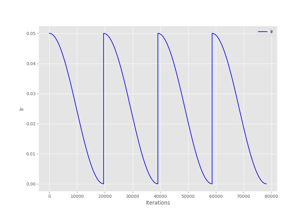
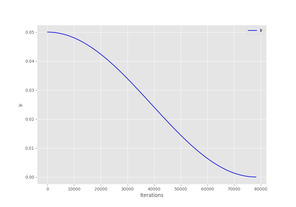
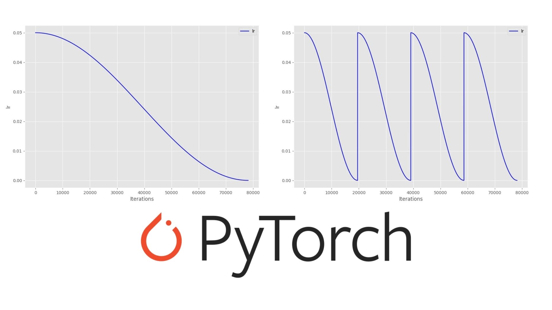
Let’s take a closer look at the above two images. Figure 2 shows the learning rate schedule when the learning rate restarts after every 50 epochs. You can see how smoothly the learning rate decreases for 50 epochs and then shoots up to 0.05. In figure 3, the learning rate keeps on decreasing evenly till 200 epochs. This is because \(T_0\) is 200 in this case (the third train run).

It is clear that the schedules have worked correctly. But what about the losses. Do we have the least validation loss in case of warm restarts or not? Let’s check that out.

The Loss Plots

We will start with the default case loss plot.

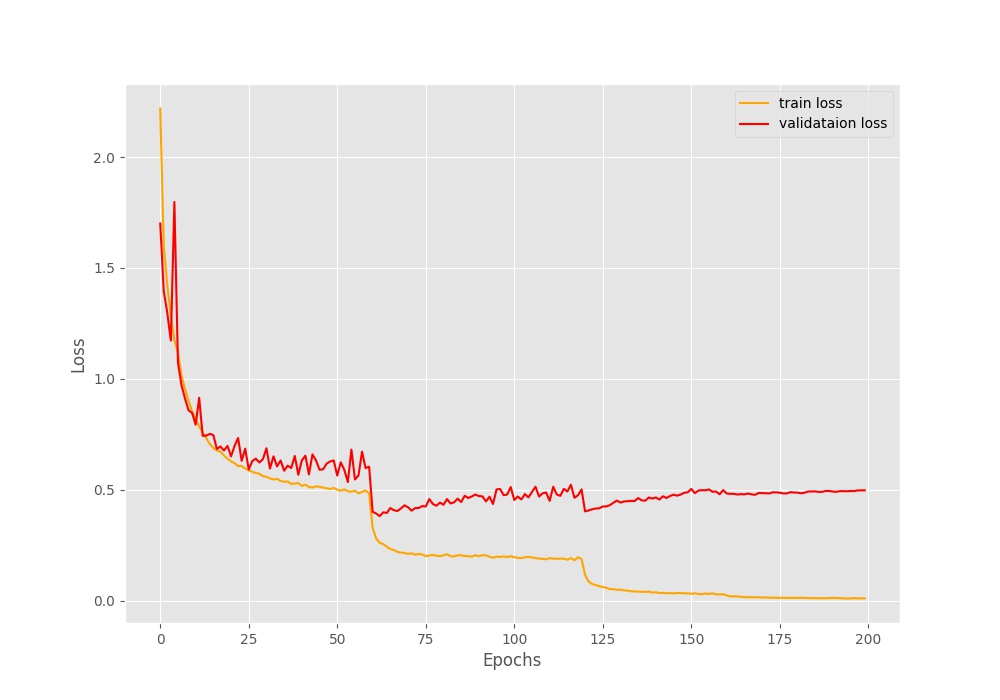
Figure 4 shows the loss for the default case where we do not use warm restarts. We can see that every time the learning rate is reduced at 60, 120, and 160 epochs, then the training loss also decreases. Interestingly, at the same time, the validation loss starts to increase. By the end of the training, we have a validation loss of somewhere around 0.5 for the default case.

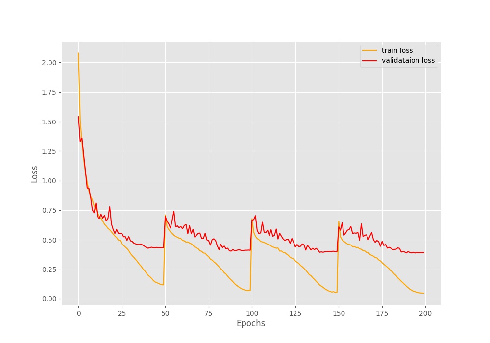
In figure 5 we see the loss for warm restarts at every 50 epochs. This time both the training and validation loss increase by a large margin whenever the learning rate restarts. But by the end of the training, the validation loss is around 0.4 which is less than that of the default case. This means that the warm restarts seem to be working.

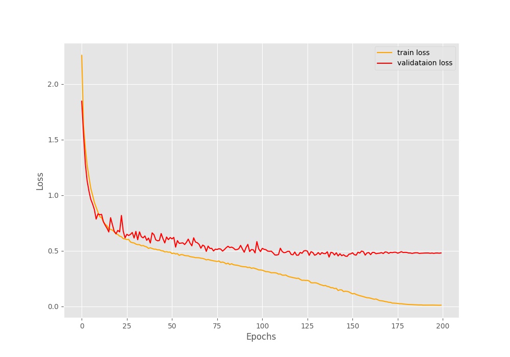
Figure 6 shows the loss when we schedule the learning rate to decrease till the end of training without any restarts. Only the Cosine Annealing keeps on reducing the learning rate. Somewhere after 175 epochs, the loss does not decrease for the training part. This is most probably because the learning rate is so low that any more learning does not happen. At the same time, the validation loss seems to increase by some amount. The final validation loss is around 0.48, which is less than the default case but more than the \(T_0 = 50\) case.

Combining the Validation Loss Plot

We will write a few lines of code to combine the validation loss plots. We already have the loss plots serialized to disk in the form .pkl files. It will be easy to deserialize and plot them.

The code here will go into the plot.py Python file.

import joblib
import matplotlib.pyplot as plt
import matplotlib

matplotlib.style.use('ggplot')

default_loss = joblib.load('outputs/val_loss.pkl')
wr_loss_s50 = joblib.load('outputs/wr_val_loss_s50_m1.pkl')
wr_loss_s200 = joblib.load('outputs/wr_val_loss_s200_m1.pkl')

plt.figure(figsize=(10, 7))
plt.plot(default_loss, color='red', label='Default validataion loss')
plt.plot(wr_loss_s50, color='green', label='T_0 = 50 validation loss')
plt.plot(wr_loss_s200, color='gray', label='T_0 = 200 validation loss')
plt.xlabel('Epochs')
plt.ylabel('Loss')
plt.legend()
plt.savefig('outputs/loss_plot_combined.jpg')
plt.show()

This is all the code we need. We are reading the .pkl files, plotting them in a single graph, and saving the plot to disk as loss_plot_combined.jpg. Execute the script.

python plot.py

Looking at the plots in the same graph will make it a lot easier for us to analyze them.

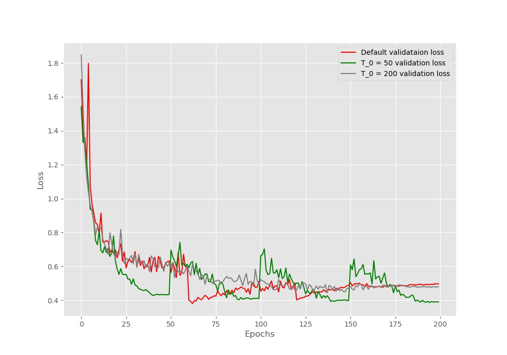
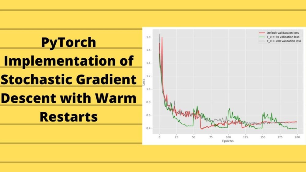
The results are pretty interesting. We can see that the default schedule (red line) loss value is the highest by the end of the training. Warm restarts of every 50 epochs is giving the least loss (green line) followed by learning rate scheduling using cosine annealing till the end of the training (gray line). This is somewhat different from the actual results posted in the SGDR paper.

In the paper, \(T_0 = 200\) scheduling gave the least loss. In our implementation, it is surely higher. Now, there may be a few reasons for this. The first obvious one being different neural network models. The authors used the Wide Residual Networks while we use the ResNet34 deep learning model.

What More Can You Do

I hope that you try training with Wide Residual Networks and share your findings in the comment section.

Summary and Conclusion

In this tutorial, you learned how to implement a small part of the SGDR: Stochastic Gradient Descent with Warm Restarts paper using PyTorch. We got to know how warm restarts affect the training and validation losses of deep neural networks and how helpful it can be. I hope that you learned something new.

If you have any doubts, thoughts, or suggestions, then please leave them in the comment section. I will surely address them.

You can contact me using the Contact section. You can also find me on LinkedIn, and Twitter.