Stochastic Gradient Descent with Warm Restarts: Paper Explanation

In this article, we will dive into the concept of Stochastic Gradient Descent with Warm Restarts in deep learning optimization and training. This is actually part 1 of two-part series.

• (This week) We will go over the paper SGDR: STOCHASTIC GRADIENT DESCENT WITH WARM RESTARTS in detail. We will learn as much as we can about the concept and experiments.
• (Next week) We will set up our PyTorch experiments to try and replicate the usefulness and claims of the paper. At least to some extent.

In particular, we will cover the following things in this article.

• An introduction to the paper.
  • What is Stochastic Gradient Descent with Warm Restarts?
  • What are its claims?
• Stochastic Gradient Descent with Warm Restarts in Detail.
  • How is Cosine Annealing used?
  • The formula for learning rate update.
• Experiments and results.
  • The training parameters and datasets used.
  • The deep learning models used.
  • Analyzing the loss graphs from the paper.
  • Single models vs. ensembles.
• Advantages of Stochastic Gradient Descent with Warm Restarts.

Introduction to Stochastic Gradient Descent with Warm Restarts

Stochastic Gradient Descent with Warm Restarts is a learning rate scheduling technique. It was introduced in the paper SGDR: STOCHASTIC GRADIENT DESCENT WITH WARM RESTARTS by Ilya Loshchilov & Frank Hutter first in 2016. Since then, it has gone many updates as well. We will go through the latest updated paper, that was submitted in 2017.

What is Stochastic Gradient Descent with Warm Restarts?

Stochastic Gradient Descent with Warm Restarts or SGDR for short is a learning rate scheduling technique. Specifically, it helps to reduce the learning rate till a certain specified epoch number. After that, the SGDR algorithm again warm restarts the learning rate. This means that it increases the learning rate to the initial value again. In turn, this helps the neural network model to converge much faster than using a static learning rate. In many cases, it also beats other scheduling techniques.

And of course, as per the paper, we have to use SGD (Stochastic Gradient Descent) with momentum optimizer with this technique.

What are some Main Claims of the Technique?

The following are some of the advantageous claims made by the authors in regard to using SGDR while training deep neural networks:

• When using warm restarts with Stochastic Gradient Descent, we can improve the deep learning model’s anytime performance.
• When using Stochastic Gradient Descent with Warm Restarts, the neural network training converges much faster when compared with the default/previous scheduling techniques.

We will get into the details of the above points and also some other advantages further into the article.

The Stochastic Gradient Descent with Warm Restarts Technique and Cosine Annealing

By now, we know that the scheduling technique restarts the learning rate at certain epochs. But how does it do so, and what are the intermediate steps the algorithm goes through. To learn about those, let’s take a look at the following image.

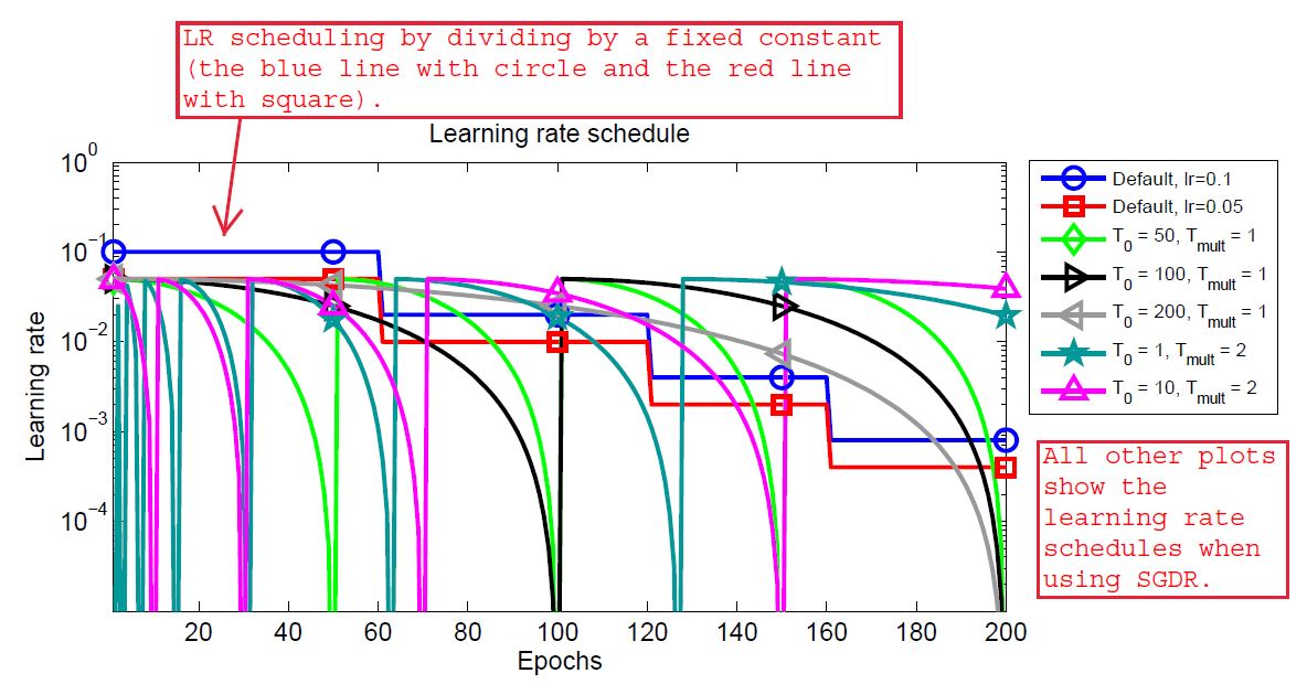
You can find the original image in the paper and I have added some text for better understanding. So, we can see a bunch of colorful plots and a lot of symbols in the adjacent box. Let’s see what all of this means.

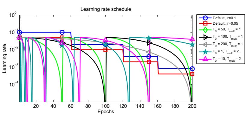
In figure 2, all the lines actually show the changing learning rates starting from epoch 0 to epoch 200. The blue line with the circle and the red line with the square shows the learning rate schedules when using the multi-step learning rate scheduling technique. These are shown to draw a contrast to the new technique, that is SGDR.

In all the other lines, we can see that the learning rates are decreasing for certain epochs and then increasing again. This is the main concept of warm restart. First, we provide an initial learning rate, then keep reducing evenly it till epoch \(T_0\), then again restart to the initial value. While restarting, we can also apply a multiplicative factor, \(T_{mult}\) which we just multiply to \(T_0\) so that it again goes through decay and restart after a certain number of increased epochs.

A Short Example

For example, let’s start with a learning rate of 0.1, \(T_0\) of 50, and \(T_{mult}\) of 1. This means that the learning rate will keep reducing till epoch 50. Then it will again increase to 0.1 from epoch 51 and it will also be multiplied with \(T_{mult}\), that is 1. So, all in all, the learning rate will restart every 50 epochs and this process will keep repeating every 50 epochs till the end of the training.

After this example, we can easily infer the image in figure 2. You can analyze all the \(T_0\) values and see how the learning rates are reducing and again restarting. Perhaps, one of the interesting ones in the figure is \(T_0 = 200\) which keeps on reducing the learning rate till the end of training without any restarts. Further in the article, we will also see, how each of the restart ranges perform while training.

The Warm Restart

But at what point does the learning rate reduce within each 50 epoch range? It keeps on reducing every batch within an epoch and restarts after every \(T_i\) epochs, where \(i\) is the index of the run.

We can understand this approach even better by quoting the authors from the paper here.

We simulate a new warmstarted run / restart of SGD once \(T_i\) epochs are performed, where \(i\) is the index of the run. Importantly, the restarts are not performed from scratch but emulated by increasing the learning rate \(\eta_t\) while the old value of \(x_t\) is used as an initial solution. The amount of this increase controls to which extent the previously acquired information (e.g., momentum) is used.

SGDR: Stochastic Gradient Descent with Warm Restarts

The above lines make us understand quite easily how to perform warm restarts while training deep neural networks.

The Learning Rate Decay

The next important part of the process is the decay of the learning rate within an epoch range. We know that the learning rate is decayed within each batch. But what is the method to do so?

The learning rate is decayed with a cosine annealing for each batch. And the following image gives the formula.

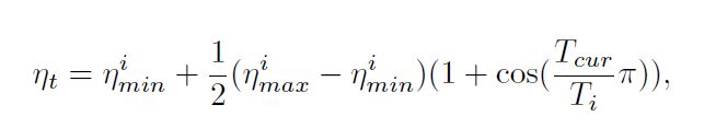
Figure 3 shows the cosine annealing formula using which we reduce the learning rate within a batch when using Stochastic Gradient Descent with Warm Restarts. In the formula, \(\eta_{min}\) and \(\eta_{max}\) are the minimum and maximum values of the learning rate. Generally, \(\eta_{max}\) is always the initial learning rate that we set. And we can change \(\eta_{min}\), that is, within an epoch range, we can choose to what value the learning rate should reduce to. \(T_{cur}\) keeps track of the number of epochs since the last warm restart and is updated at each batch iteration \(t\).

There are many other details in the paper regarding formula. You can give a read to Section 3 of the paper to know more. Next, we will move on to analyzing the experimental results from the paper.

Experiments and Results

The authors describe their experiments and results on the CIFAR-10, CIFAR-100, an EEG dataset, and a smaller version of the ImageNet dataset.

For the sake of brevity, we will focus on the results of CIFAR-10 and CIFAR-100 mostly in this article.

Experiment Settings and the Hyperparameters

First, let’s go over the settings and hyperparameters for the experiments and training. We are focusing on the CIFAR-10 and CIFAR-100 datasets here.

The authors use the SGD optimizer with an initial learning rate of 0.05, weight decay of 0.0005, set the dampening to 0, momentum to 0.9. The minibatch size is 128. They also use horizontal flipping and random cropping as augmentations for the CIFAR-10 and CIFAR-100 images.

For comparison, the authors of the paper reproduce the results of Zagoruyko & Komodakis (2016) with the same settings, except for one change. They compare their SGDR scheduling results with step learning rate scheduling results of Zagoruyko & Komodakis (2016) where they reduce the learning rate by a factor of 0.2 every 60, 120, and 160 epochs. You may ask, “why to compare with the results of Zagoruyko & Komodakis (2016)?” Because Ilya Loshchilov & Frank Hutter use the same network architecture as introduced by Zagoruyko & Komodakis (2016) in their paper Wide Residual Networks.

This brings us to our next topic, that is the model used for training.

The Neural Network Architecture

For the SGDR experiments, Ilya Loshchilov & Frank Hutter use the Wide Residual Networks (WRNs) for training. We denote them as WRN-d–k, where d is the depth and k is the width of the network. And for the SGDR experiments, the models are WRN-28-10, and WRN-28-20.

Test Error Results for Single Models

It’s time to analyze the performance of SGDR. We will start with the error plots.

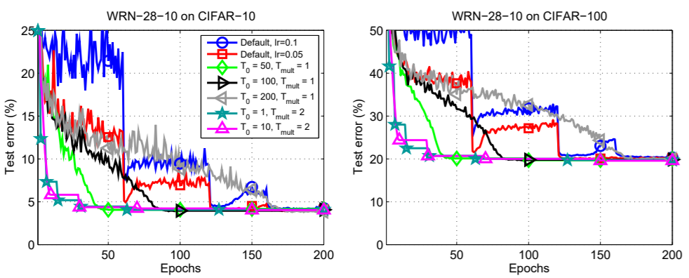
In figure 4, we can clearly see that the SGDR test errors are lower in all cases. The default error plots are those from Ilya Loshchilov & Frank Hutter experiments replication. They are the blue and the red lines.

Perhaps, the most amazing part is, the SGDR test error is almost always lower than the default errors at any point on the graph. If not, then it becomes better by the end of the training. This is true for both the datasets, which are CIFAR-10 and CIFAR-100 (left and right graphs respectively).

We can infer some of the things even better by looking at the zoomed-in images of the above plots.

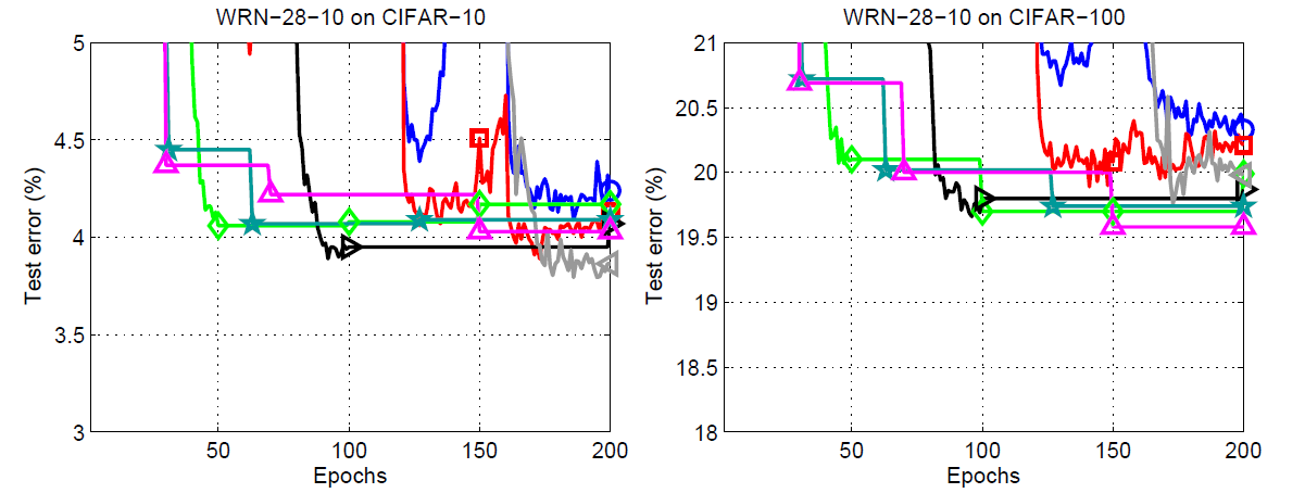
We can see something really interesting in the zoomed plot for the CIFAR10 dataset. We are getting the best results, when \(T_0 = 200\) with the multiplication factor 1. That is, we do not restart the learning rate at all but keep on reducing it uniformly until the end of the training. And for the CIFAR100 dataset. \(T_0 = 10\) and \(T_{mult} = 2\) are giving the best results. This means we do the first warm restart at epoch 10, then keep on doubling the restart period.

Also, with the CIFAR-100 dataset, the test error margin between stochastic gradient descent with warm restarts training and the default cases are higher than the CIFAR-10 dataset. This could mean that the SGDR training performs well even when the complexity of the dataset increases.

Now, coming to test error results of even wider neural networks within WRN family. The authors have also included the results for WRN-28-20.

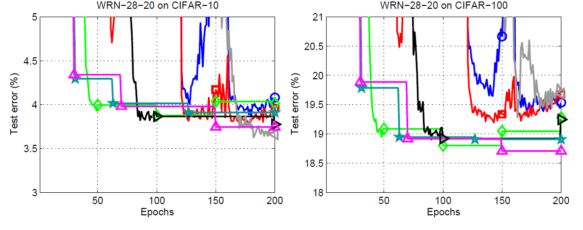
Figure 6 shows the results for the WRN-28-20 test errors. This time also a single run SGDR with \(T_0 = 200\) gives the best results on the CIFAR-10 dataset. But the following line by the authors sums up a pretty important thing about the single run models.

However, the same setting with \(T0 = 200\) leads to the worst anytime performance except for the very last epochs.

SGDR: Stochastic Gradient Descent with Warm Restarts

If we pick any of the SGDR run models, then every other model gives better results at any point during training except the single run model. But then again, the single run model, that is \(T_0 = 200\), gives the best results by the end of 200 epochs.

Next up focusing a bit more on the SGDR runs where \(T_{mult} = 2\). We can see that there are two runs for these, that is \(T_0 = 1\) and \(T_0 = 10\). And both of them reach very low test errors pretty quickly. In fact, that was the aim of the authors as well. Starting with a very early restart and doubling the epochs for the restarts does actually help reach the low test errors pretty quickly. In fact, the \(T_0 = 10, T_{mult} = 2\) gives the second best test errors on the CIFAR-10 dataset and the best results on the CIFAR-100 dataset.

There is one more interesting thing to note in the case of WRN-28-20. If you observe closely, then using the learning rate reduction technique of SGDR, the \(T_0 = 50\) run beats the respective WRN-28-10 even before the first restart. This means that increasing the width of WRNs coupled with the learning rate decay of SGDR can prove to be very useful in converging the models really fast.

One last thing in the case of single model runs before moving on to the ensemble models.

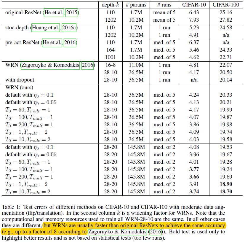
The above figure shows the results for different runs in a tabular format. We will not go into much detail of that as I hope everything can be inferred easily by just going through each row.

Test Error Results for Ensembles

We will go over the ensemble model results in brief here. The ensemble model results were not in the original (first) publication. It was later added in future updates.

Before moving ahead, all the ensemble model results are with \(T_0 = 10, T_{mult} = 2\) SGDR runs. Also, the architecture in all cases is WRN-28-10. Let’s take a look at the figure of a table from the paper.

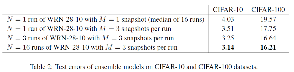
In figure 8, we can see that one of the ensemble results (the last row) is giving the lowest test errors among all the ensemble and single models as well. But what are N, M, and snapshots?

Here, N is the number of runs or the number of times the model has been trained. But we do not consider the ensembling as per the runs. Instead, the author chose a different method. They selected models to ensemble at different snapshots within a single run. Specifically, M number of snapshots are made at epochs 30, 70, and 150. As the \(T_0 = 10, T_{mult} = 2\), so, these snapshots are just before the learning rate becomes zero. For calculation, the authors aggregate the probabilities of softmax layers of the snapshots at epoch indices.

Now, let’s take a look at another figure.

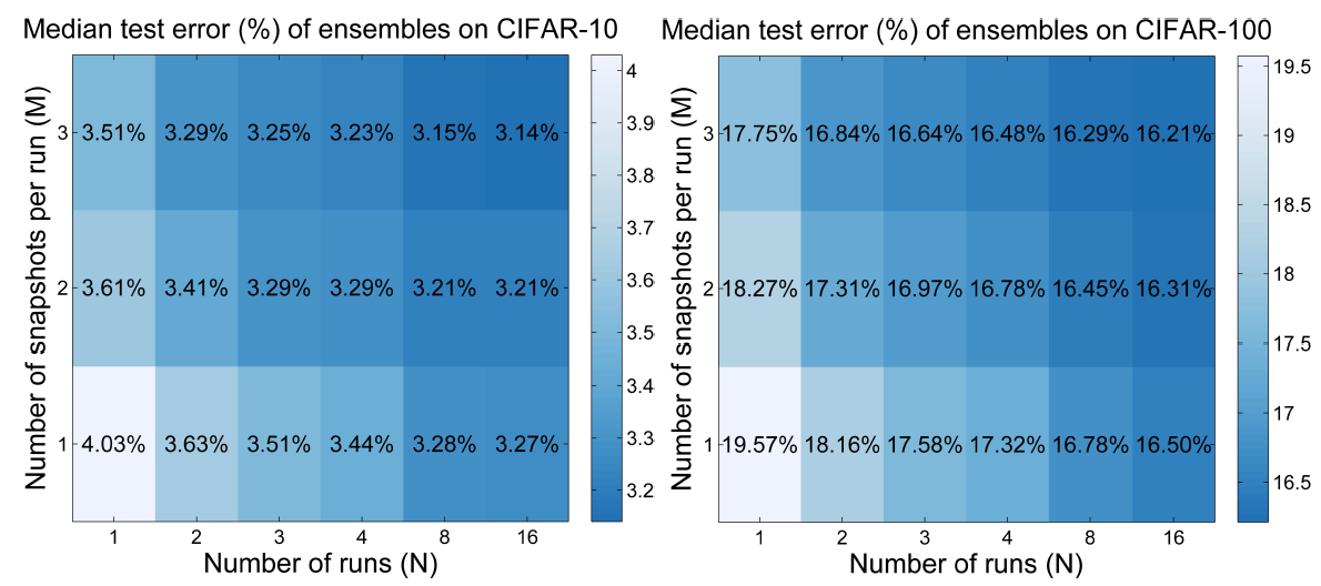
Figure 9 shows the number of runs vs. number of snapshots matrix for the CIFAR-10 and CIFAR-100 dataset. Quoting the authors here sums up the results from above quite beautifully.

The original test error of 4.03% on CIFAR-10 and 19.57% on CIFAR-100 (median of 16 runs) can be improved to 3.51% on CIFAR-10 and 17.75% on CIFAR-100 when M = 3 snapshots are taken at epochs 30, 70 and 150: when the learning rate of SGDR with \(T_0 = 10; T_{mult} = 2\) is scheduled to achieve 0 … and the models are used with uniform weights to build an ensemble.

SGDR: Stochastic Gradient Descent with Warm Restarts

This shows that we can ensemble models without training multiple models simultaneously and taking snapshots within that single run as well. This can greatly improve training time and we can get faster results as well.

The paper also goes into more details when training on an EEG dataset and even the small ImageNet dataset. But we will end our discussion of the results here and I hope that you give the paper a read to know more about the results.

Advantages of Stochastic Gradient Descent with Warm Restarts

By now, we know many advantages of training with SGDR. Let’s sum those up.

• Using the SGDR scheduling technique while training, we can achieve almost anytime better performance of a neural network. When compared to default scheduling technique, SGDR tends to provide much better results.
• If we can choose the restart period and multiplicative factor wisely, then the model can reach pretty low test error within the first few epochs only. This means that the neural network may converge much faster than when not using SGDR.
• We can also get ensembles out of models by taking snapshots at the right time even within a single run. This means that for a single training run, we can easily get multiple models to ensemble.

In the next article, we will try and implement a small part of the paper using PyTorch to get an idea of the experiments and the results.

Summary and Conclusion

In this article, you got to learn about Stochastic Gradient Descent with Warm Restarts. We went through the technique, the models, and the advantages of using SGDR while training large neural networks.

I hope that you learned something new from this article. If you have any doubts, thoughts, or suggestions, then please leave them in the comment section. I will surely address them.

You can contact me using the Contact section. You can also find me on LinkedIn, and Twitter.