
In the last two tutorials, we have been dealing with medical image datasets. In one of the previous posts, we trained a custom image classification model using PyTorch on the Medical MNIST dataset. And in the previous post, we used the Medical MNIST pretrained model to classify Pneumothorax images. And if you have gone through the previous post or intend to go through it, then you will find out that we did not get much success there. The model was overfitting very soon and the accuracy and the F1-score metrics were plateauing from the second epoch. In this tutorial, we will try to rectify that and build a much better model. We will try to solve the Pneumothorax Binary Classification with PyTorch using Oversampling of the negative class.
Medical imaging classification is a difficult problem in itself. On top of that, when the data is highly imbalanced, it causes even more issues. The deep learning model tends to overfit a single class very easily and does not learn the features of the other class. In our case, the Pneumothorax Binary Classification task does not contain enough negative class images. So, in our previous training experiment, the model predicted each image as pneumothorax during inference.
In this post, we will again try to solve the Pneumothorax binary classification problem using PyTorch. But with a new strategy. We will oversample the negative classes first, and then move over to training the model again.
Points to Cover in This Post
This post will not cover much training code. Almost all of the code from the previous tutorial is reusable. Still, there are important steps to cover here.
- We will have a Jupyter Notebook which will cover the oversampling code for the negative classes. This notebook will also create a separate test set for final testing of our trained model.
- We will also cover a few experiments under similar settings for the original dataset. This is mainly needed as the previous post’s training strategy was just a bit different.
- There is a new test script in this post that we will write that will give us the final binary accuracy, F1-score, and the confusion matrix on the test set.
We will use the same Medical MNIST PyTorch pretrained model for Pneumothorax binary classification problem with oversampling. This will give us a pretty accurate picture of how helpful our approach is to solve the problem.
Approach We Will Take in This Post
As discussed above, a lot of Python code files are directly reusable from the previous post. So, we will skip the parts that are entirely similar. For coding discussion, we will cover the following things:
- A Jupyter Notebook covering the oversampling code for negative classes and creating the test test.
- The dataset preparation Python script. As the directory structure of the dataset is changing, so our dataset preparation code will change. We will discuss that.
- The test script that will test the final trained model.
The Directory Structure
Understanding the directory structure for this project is going to be pretty important. Let’s take a look at that.
├── input
│   ├── pneumothorax-binary-classification-task
│   │   ├── small_train_data_set
│   │   │   └── small_train_data_set [2028 entries exceeds filelimit, not opening dir]
│   │   └── train_data.csv
│   ├── processed_data
│   │   ├── test
│   │   │   ├── normal [50 entries exceeds filelimit, not opening dir]
│   │   │   └── pneumothorax [50 entries exceeds filelimit, not opening dir]
│   │   └── train_valid
│   │       ├── normal [1670 entries exceeds filelimit, not opening dir]
│   │       └── pneumothorax [1547 entries exceeds filelimit, not opening dir]
│   └── medical_mnist_pretrained.pth
├── notebooks
│   ├── simple_training_outputs
│   │   ├── accuracy.png
│   │   ├── heatmap.png
│   │   ├── loss.png
│   │   ├── model.pth
│   │   ├── score.png
│   │   ├── test_image_24.png
│   │   ├── test_image_48.png
│   │   └── test_image_72.png
│   ├── pneumothorax_simple_binary_classification.ipynb
│   └── preprocess_and_oversample.ipynb
├── outputs
│   ├── accuracy.png
│   ├── f1_score.png
│   ├── heatmap.png
│   ├── loss.png
│   ├── model.pth
│   ├── test_image_24.png
│   ├── test_image_48.png
│   ├── test_image_72.png
│   └── test_image_96.png
|── src
    ├── datasets.py
    ├── model.py
    ├── test.py
    ├── train.py
    └── utils.py
Let’s understand the above structure in detail.
input: This contains two subdirectories. Thepneumothorax-binary-classification-taskis the original dataset directory that we used in the previous post. And theprocessed_datais the new dataset that we will create in this post. Basically, the new data contains new augmentated images for the negative classes and divides the dataset into atrain_validdirectory and atestdirectory. It also contains themedical_mnist_pretrained.pthPyTorch weights that we used in the previous post. As you might be knowing we had trained a custom CNN on the Medical MNIST dataset and are loading those weights and fine-tuning them.notebooks: Thenotebooksdirectory contains two notebooks.preprocess_and_oversample.ipynbto create the new oversampled dataset andpneumothorax_simple_binary_classification.ipynbto train the original dataset using the same model so that we will have some comparisons to make. We already carried out the training in the previous post. But this notebook follows similar strategy as this post on the original dataset. It also runs a test using the trained model and we will discuss those things further on. Thesimple_training_outputscontains the outputs from thepneumothorax_simple_binary_classification.ipynbnotebook.outputs: This directory contains all the outputs that this post’s training and testing script will generate.src: As usual, this contains all the source code.
Except for the dataset, you will get all the Python files, notebooks, and pretrained models while downloading the zip file for this post. You can download the original Pneumothorax binary classification dataset here for PyTorch training experiments. We will write the code to generate the new dataset.
Training Results without Oversampling
As you know the pneumothorax_simple_binary_classification.ipynb notebook contains the training and testing results on the original Pneumothorax dataset. Although we will not go into the coding details, going over a few important technical details will help.
We trained the same model on the same dataset in the previous post also. So, why another notebook here?
This is mainly to replicate the process that we are following in the oversampling method. In the previous post, we had a training and validation set for the training pipeline. Then we used images from the internet for inference. Instead of that, in the current notebook, we are using 70% data for training, 15% for validation, and 15% for final testing.
We will discuss the following points shortly for the simple training process without oversampling:
- The training and validation accuracy.
- The training and validation loss.
- F1-score for training and validation.
- The final test results along with the confusion matrix.
Before getting into the results, let’s take a look at the training settings and hyperparameters.
- We are resizing the images to 256×256 dimensions and applying center cropping using the transforms.
- The batch size is 16.
- We train for 100 epochs with initial learning rate of 0.0001.
- The Cosine Annealing scheduler warm restarts the learning rate every 25 epoch.
Accuracy, Loss, and F1-Score for Training and Validation
During the training, there were 1418 training images and 517 validation images.
After training for 100 epochs, the final validation accuracy is 79.110% with an F1-score of 0.883. And the final validation loss is 0.503.
The following are the graphs for all three.
The training and the F1-score values are plateauing very soon.
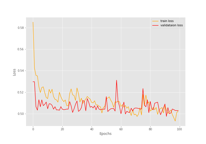
The training loss values seem to be decreasing till the end of training but are still not very promising.
Most probably, during evaluation, the model is just predicting the same values every time due to the uneven distribution of the dataset.
The Confusion Matrix
For the final testing, along with the binary accuracy and F1-score, we also plot the confusion matrix. The test set had 92 images. The test accuracy was 78.261% with an F1-score of 0.878.
This number looks good until we take a look at the confusion matrix.
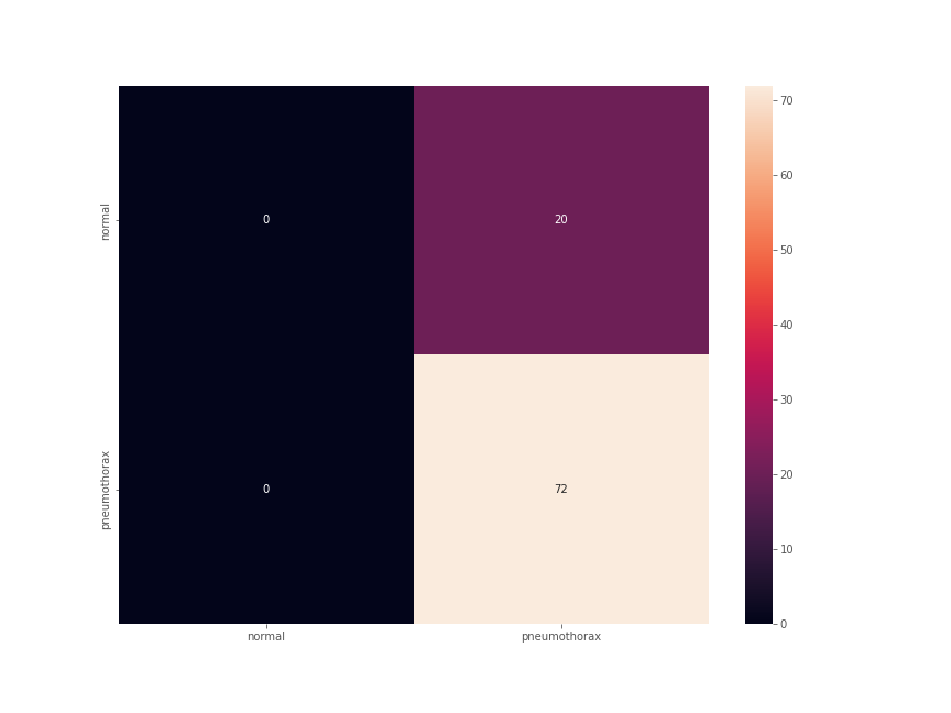
This is interesting. Out of the 72 Pneumothorax images, all 72 were predicted correctly. This is good. But along with that 20 normal lung x-ray images were also predicted as Pneumothorax. None of the normal images were predicted correctly.
This is a classic case of a deep learning model overfitting on a single class because of an imbalanced dataset. Now, in deep learning image classification for medical imaging, it is true that we need to predict the positive disease cases correctly. But that does not mean every negative case should also be predicted as positive.
So, how do we correct the above situation? And even if it’s possible, to what extent can we improve the model? Will the approach that we are taking in this post further help? Let’s find that.
From the next section onward, we will completely focus on the new approach that we are applying for the Pneumothorax binary classification using PyTorch.
Pneumothorax Binary Classification with PyTorch using Oversampling
In this section, we will start with the discussion of the notebook that prepares the dataset, then move on to the Python files for training, validation, and testing.
The Data Preparation Notebook
The preprocess_and_oversample.ipynb notebook inside the notebooks directory does three important things:
- Oversamples the negative class images by applying random augmentation.
- Creates a new
processed_datasubdirectory inside theinputdirectory to keep the entire Pneumothorax binary classification dataset in a bit different format. - Divides the dataset into training/validation and a test set.
We will cover the above points in detail while going through the code in the notebook.
Now, let’s discuss the content of the preprocess_and_oversample.ipynb.
Starting with the imports and setting the seed.
import torch
import cv2
import os
import tqdm
import glob as glob
import pandas as pd
import shutil
import matplotlib.pyplot as plt
import numpy as np

from tqdm.auto import tqdm
from torchvision import transforms

SEED = 42
np.random.seed(SEED)
torch.manual_seed(SEED)
Setting the seed is quite important as we want PyTorch to apply the same set of augmentations each time. We use the transforms from torchvision to augment the normal x-ray images, oversample them, and save them to disk.
Make New Directories for Training and Validation Set
Inside the input directory, we will create a processed_data subdirectory that will in turn contain another train_valid subdirectory. This will store the images for training and validation.
# Create new directories to store the new dataset.
processed_dir = '../input/processed_data/train_valid'
os.makedirs(processed_dir, exist_ok=True)

# Create class subdirectories.
pneumothorax = f"{processed_dir}/pneumothorax"
normal = f"{processed_dir}/normal"

os.makedirs(pneumothorax, exist_ok=True)
os.makedirs(normal, exist_ok=True)
The positive class images will go into the pneumothorax directory and the negative class images will go into the normal directory.
Read the Images and Copy Them to the New Directories
This is a simple code block. This will read the CSV file, map each image to the original file in the directory, and copy the images as per the classes to the new directories.
ROOT_PATH = '../input/pneumothorax-binary-classification-task/'
df = pd.read_csv(f"{ROOT_PATH}/train_data.csv")

for i in tqdm(range(len(df)), total=len(df)):
    file_name = df.file_name[i]
    target = df.target[i]

    image_path = f"{ROOT_PATH}/small_train_data_set/small_train_data_set/{file_name}"
    if target == 1:
        dest_path = f"{pneumothorax}/{file_name}"
    else:
        dest_path = f"{normal}/{file_name}"

    shutil.copy(image_path, dest_path)
Augment All Normal Lung X-Ray Images
This is the important oversampling part. We will define two different transforms and apply the augmentations to all the negative class images.
transform1 = transforms.Compose([
    transforms.ToPILImage(),
    transforms.RandomHorizontalFlip(p=1.0),
])

transform2 = transforms.Compose([
    transforms.ToPILImage(),
    transforms.RandomAutocontrast(p=1.0)
])
We have two different transforms in the above code block. One is for horizontally flipping the images and another to apply random contrast to images.
Note that we are passing a probability of 1.0 which ensures all augmentation will be applied to all the images.
The next code block applies flip augmentation to the current 430 images.
all_images = glob.glob(f"{normal}/*")
print(all_images[:5])
print(len(all_images))

# Augment all the current images.
for i, image_path in tqdm(enumerate(all_images), total=len(all_images)):
    image = cv2.imread(image_path, cv2.IMREAD_UNCHANGED)
    tfms_image = transform1(image)
    tfms_image = np.array(image)
    cv2.imwrite(f"{normal}/transformed_1_{i}.png", tfms_image)
After this augmentation is complete we have 860 negative class images with us now. This is around half as that of the positive class images.
Now, let’s apply random contrast augmentation to these 860 images.
# Again augment eveyrthing.
all_images = glob.glob(f"{normal}/*")

for i, image_path in tqdm(enumerate(all_images), total=len(all_images)):
    image = cv2.imread(image_path, cv2.IMREAD_UNCHANGED)
    tfms_image = transform2(image)
    tfms_image = np.array(image)
    cv2.imwrite(f"{normal}/transformed_2_{i}.png", tfms_image)
After the above augmentation step is complete, we will have 1720 negative class images with us. This is just over 100 images more than the positive classes and should be perfect for our oversampling experiments.
Prepare the Test Set
Now, the final part of the data preparation step is to create a test set that will not be used during training and validation iterations. We will set out 50 normal images and 50 pneumothorax images for testing. Simply, we will create a test directory inside input/processed_data and copy the images to the respective class folders.
test_dir = '../input/processed_data/test'
os.makedirs(test_dir, exist_ok=True)

test_dir_pneumothorax = f"{test_dir}/pneumothorax"
test_dir_normal = f"{test_dir}/normal"

os.makedirs(test_dir_pneumothorax)
os.makedirs(test_dir_normal)

# Move 50 normal images to test_dir
all_normal_images = os.listdir(normal)
print(len(all_normal_images))
print(all_normal_images[:3])

for i, image in enumerate(all_normal_images):
    if i == 50:
        break
    shutil.move(f"{normal}/{image}", f"{test_dir_normal}/{image}")

# Move 50 pneumpothorax images to test_dir
all_pneumothorax_images = os.listdir(pneumothorax)
print(len(all_pneumothorax_images))
print(all_pneumothorax_images[:3])

for i, image in enumerate(all_pneumothorax_images):
    if i == 50:
        break
    shutil.move(f"{pneumothorax}/{image}", f"{test_dir_pneumothorax}/{image}")
Now, our entire oversampled data preparation step is complete.
Now, let’s move on to the Python code files.
The Python Scripts
In the Python code files, the utils.py, model.py, and train.py are the same as the previous tutorial. So, we will not go over them again. They are very simple Python files. If you go through the previous tutorial, you will be able to understand them easily.
Now, because the dataset directory structure has changed, the code for datasets.py will change. Another new script is the test.py which we will cover after the training part is complete.
Although the dataset preparation code is simple, because it covers a few important parameters, let’s go over it.
Preparing the Training and Validation PyTorch Datasets
The dataset and data loader preparation code will go into the datasets.py file.
Starting with the imports and defining a few important constants.
import torch

from torchvision import datasets, transforms
from torch.utils.data import DataLoader, Subset

# Required constants.
ROOT_DIR = '../input/processed_data/train_valid'
VALID_SPLIT = 0.15
RESIZE_TO = 256 # Image size of resize when applying transforms.
BATCH_SIZE = 32
NUM_WORKERS = 4 # Number of parallel processes for data preparation.
As you may observe, we are using 15% of the data for validation and the rest for training. Now, one major thing to note here is the image resizing constant. We will be resizing the images to 256×256 dimensions during the transforms. And then apply center cropping to reduce the dimension to 224×224. This will help us remove the area around the border of the image and outside of the lung periphery whose information the model does not need.
The batch size is 32 and the number of parallel workers is 4.
The next code block covers the training and validation transforms.
# Training transforms
def get_train_transform(RESIZE_TO):
    train_transform = transforms.Compose([
        transforms.Resize((RESIZE_TO, RESIZE_TO)),
        transforms.CenterCrop((224, 224)),
        transforms.ToTensor(),
        transforms.Normalize(
            mean=[0.5, 0.5, 0.5],
            std=[0.5, 0.5, 0.5]
            )
    ])
    return train_transform

# Validation transforms
def get_valid_transform(RESIZE_TO):
    valid_transform = transforms.Compose([
        transforms.Resize((RESIZE_TO, RESIZE_TO)),
        transforms.CenterCrop((224, 224)),
        transforms.ToTensor(),
        transforms.Normalize(
            mean=[0.5, 0.5, 0.5],
            std=[0.5, 0.5, 0.5]
            )
    ])
    return valid_transform
We are not performing any major augmentation here. As discussed, we are cropping the image to 224×224 dimensions for both, the training set and the validation set.
Now, the final code block contains the functions to prepare the datasets and data loaders.
def get_datasets():
    """
    Function to prepare the Datasets.

    Returns the training and validation datasets along
    with the class names.
    """
    dataset = datasets.ImageFolder(
        ROOT_DIR,
        transform=(get_train_transform(RESIZE_TO))
    )
    dataset_test = datasets.ImageFolder(
        ROOT_DIR,
        transform=(get_valid_transform(RESIZE_TO))
    )
    dataset_size = len(dataset)

    # Calculate the validation dataset size.
    valid_size = int(VALID_SPLIT*dataset_size)
    # Radomize the data indices.
    indices = torch.randperm(len(dataset)).tolist()
    # Training and validation sets.
    dataset_train = Subset(dataset, indices[:-valid_size])
    dataset_valid = Subset(dataset_test, indices[-valid_size:])

    return dataset_train, dataset_valid, dataset.classes

def get_data_loaders(dataset_train, dataset_valid):
    """
    Prepares the training and validation data loaders.

    :param dataset_train: The training dataset.
    :param dataset_valid: The validation dataset.

    Returns the training and validation data loaders.
    """
    train_loader = DataLoader(
        dataset_train, batch_size=BATCH_SIZE,
        shuffle=True, num_workers=NUM_WORKERS
    )
    valid_loader = DataLoader(
        dataset_valid, batch_size=BATCH_SIZE,
        shuffle=False, num_workers=NUM_WORKERS
    )
    return train_loader, valid_loader
With this, we complete the code for dataset preparation.
Training the Neural Network Model
Before we start the training, let’s discuss some of the learning parameters and settings.
- We will be loading the Medical MNIST pretrained weights into the
CustomCNNarchitecture. - The optimizer is going to be AdamW with an initial learning rate of 0.0001.
- We are using
CosineAnnealingWarmRestartslearning rate scheduler in the training code. The learning rate restart epochs is set to 50.
With the above aspects in mind, let’s start the training. Open your terminal/command line in the src directory and execute the following command.
python train.py --epochs 400 --learning-rate 0.0001
We are training the model for 400 epochs. If you are training locally, then depending on your hardware, it may take some time to complete.
The following block shows the truncated terminal outputs after the training is complete.
[INFO]: Number of training images: 2735
[INFO]: Number of validation images: 482
Computation device: cuda
Learning rate: 0.0001
Epochs to train for: 400

421,441 total parameters.
421,441 training parameters.
Epoch     0: adjusting learning rate of group 0 to 1.0000e-04.
[INFO]: Epoch 1 of 400
Training
100%|██████████████████████████████████████████████████████████████████████████████████████████████████████████████████████████| 86/86 [00:07<00:00, 10.83it/s]
Validation
100%|██████████████████████████████████████████████████████████████████████████████████████████████████████████████████████████| 16/16 [00:01<00:00, 11.47it/s]
Training loss: 0.746, training acc: 51.664, training f1-score: 0.487
Validation loss: 0.687, validation acc: 56.224, validation f1-score: 0.552
LR at end of epoch 1 9.990361684994305e-05
--------------------------------------------------
[INFO]: Epoch 2 of 400
Training
100%|█████████████████████████████████████████████████████████████████████████████████████████████████████████████████████████| 86/86 [00:06<00:00, 12.64it/s]
Validation
100%|██████████████████████████████████████████████████████████████████████████████████████████████████████████████████████████| 16/16 [00:01<00:00, 12.09it/s]
Training loss: 0.706, training acc: 53.565, training f1-score: 0.496
Validation loss: 0.674, validation acc: 59.544, validation f1-score: 0.365
LR at end of epoch 2 9.961030026748915e-05
--------------------------------------------------
...
[INFO]: Epoch 399 of 400
Training
100%|█████████████████████████████████████████████████████████████████████████████████████████████████████████████████████████| 86/86 [00:06<00:00, 12.69it/s]
Validation
100%|█████████████████████████████████████████████████████████████████████████████████████████████████████████████████████████| 16/16 [00:01<00:00, 12.29it/s]
Training loss: 0.048, training acc: 98.757, training f1-score: 0.987
Validation loss: 0.293, validation acc: 92.324, validation f1-score: 0.908
LR at end of epoch 399 1.009706434829838e-07
--------------------------------------------------
[INFO]: Epoch 400 of 400
Training
100%|█████████████████████████████████████████████████████████████████████████████████████████████████████████████████████████| 86/86 [00:06<00:00, 12.69it/s]
Validation
100%|█████████████████████████████████████████████████████████████████████████████████████████████████████████████████████████| 16/16 [00:01<00:00, 12.31it/s]
Training loss: 0.050, training acc: 98.611, training f1-score: 0.986
Validation loss: 0.293, validation acc: 92.324, validation f1-score: 0.908
LR at end of epoch 400 1.33445159034018e-11
--------------------------------------------------
TRAINING COMPLETE
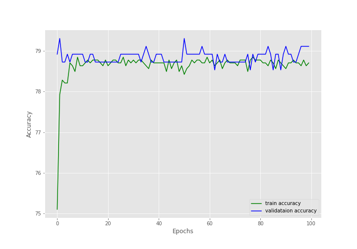
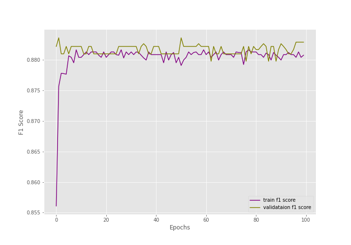
The final epochs validation loss is 0.293, validation accuracy is 92.3% and F1-score is 0.908. This looks like a good improvement compared to the simple method without oversampling. But looking at the metrics and loss graphs will be much more useful.
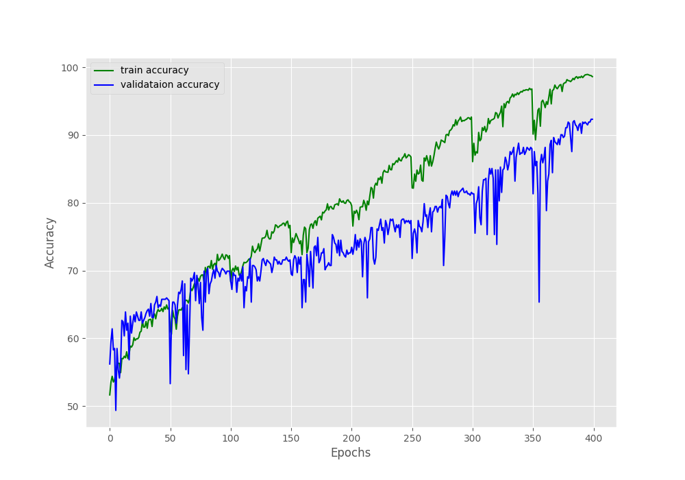
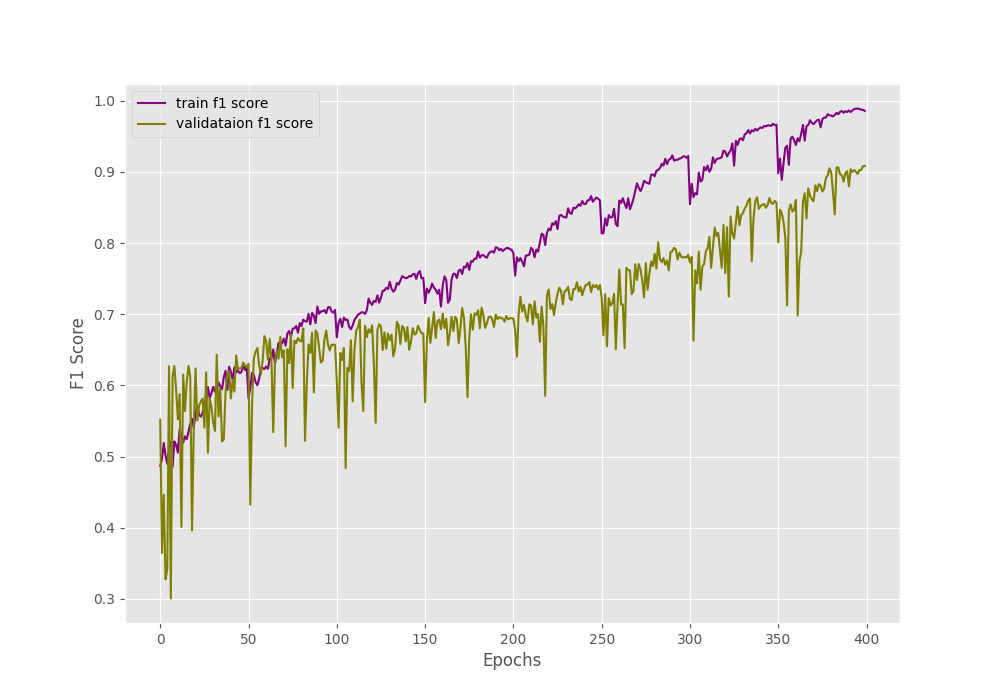
We can clearly see the dip and spike on both of the above graphs. And this is mostly happening every 50 epochs when the learning rate becomes 0 and again rises to the default value. Still, it seems like the learning rate scheduler is helping the accuracy and the F1-score to improve till the end of training.
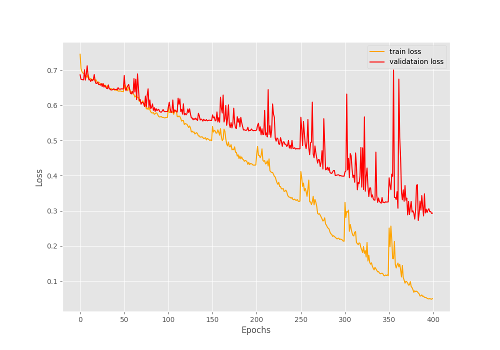
The training and validation loss values also seem to be improving till the end of training.
These results look much better than the previous case, where all the validation plots were almost not improving at all.
Running the test script will give us a much better idea.
The Test Script
Here, we will write a very simple test script to test our trained model on the held-out set. It is going to be pretty straightforward and simple. And most of the things will remain similar to the Medical MNIST test script.
The code for the test script will go into the test.py file.
The first code block contains the import statements and the constants.
import torch
import numpy as np
import matplotlib.pyplot as plt
import seaborn as sns
import cv2
from model import CustomCNN

from torchvision import transforms, datasets
from torch.utils.data import DataLoader
from tqdm.auto import tqdm
from sklearn.metrics import confusion_matrix, f1_score
from utils import (
    get_outputs_binary_list,
    count_correct_binary_pred,
    calculate_f1_score
)
# Constants and other configurations.
TEST_DIR = '../input/processed_data/test'
BATCH_SIZE = 1
DEVICE = torch.device('cuda:0' if torch.cuda.is_available() else 'cpu')
RESIZE_TO = 256
NUM_WORKERS = 4
CLASS_NAMES = ['normal', 'pneumothorax']
We define the:
- Test directory path.
- The batch size, which is 1 here as we will iterate over one image at a time.
- Again, we will follow the same resizing and cropping steps along with 4 parallel workers.
- We also define a list containing the class names that will help us map the predictions and ground truth labels to the actual class names.
Next, the functions for creating the transforms, the test dataset, and the test data loader.
def test_transform(IMAGE_RESIZE):
    transform = transforms.Compose([
            transforms.Resize((IMAGE_RESIZE, IMAGE_RESIZE)),
            transforms.CenterCrop(224),
            transforms.ToTensor(),
            transforms.Normalize(
                mean=[0.5, 0.5, 0.5],
                std=[0.5, 0.5, 0.5]
                )
        ])
    return transform

def create_test_set():
    dataset_test = datasets.ImageFolder(
        TEST_DIR,
        transform=(test_transform(RESIZE_TO))
    )
    return dataset_test

def create_test_loader(dataset_test):
    test_loader = DataLoader(
        dataset_test, batch_size=BATCH_SIZE,
        shuffle=False, num_workers=NUM_WORKERS
    )
    return test_loader
Now, the function to save the test results which we already defined in the Medical MNIST training post.
def save_test_results(tensor, target, output_class, counter):
    """
    This function will save a few test images along with the
    ground truth label and predicted label annotated on the image.

    :param tensor: The image tensor.
    :param target: The ground truth class number.
    :param output_class: The predicted class number.
    :param counter: The test image number.
    """
    # Move tensor to CPU and denormalize
    image = torch.squeeze(tensor, 0).cpu().numpy()
    image = image / 2 + 0.5
    image = np.transpose(image, (1, 2, 0))
    # Convert to BGR format
    image = cv2.cvtColor(image, cv2.COLOR_RGB2BGR)
    gt = target.cpu().numpy()
    cv2.putText(
        image, f"GT: {CLASS_NAMES[int(gt)]}",
        (5, 25), cv2.FONT_HERSHEY_SIMPLEX,
        0.7, (0, 255, 0), 2, cv2.LINE_AA
    )
    cv2.putText(
        image, f"Pred: {CLASS_NAMES[int(output_class)]}",
        (5, 55), cv2.FONT_HERSHEY_SIMPLEX,
        0.7, (0, 255, 0), 2, cv2.LINE_AA
    )
    cv2.imwrite(f"../outputs/test_image_{counter}.png", image*255.)
The test function to iterate over the test loader.
def test(model, testloader, DEVICE):
    """
    Function to test the trained model on the test dataset.

    :param model: The trained model.
    :param testloader: The test data loader.
    :param DEVICE: The computation device.

    Returns:
        predictions_list: List containing all the predicted class numbers.
        ground_truth_list: List containing all the ground truth class numbers.
        acc: The test accuracy.
    """
    model.eval()
    print('Testing model')
    test_running_correct = 0
    y_true = []
    y_pred = []
    counter = 0
    with torch.no_grad():
        for i, data in tqdm(enumerate(testloader), total=len(testloader)):
            counter += 1

            image, labels = data
            image = image.to(DEVICE)
            labels = labels.type(torch.float32).to(DEVICE)
            # Forward pass.
            outputs = model(image)

            # Get the binary predictions, 0 or 1.
            outputs_binary_list = get_outputs_binary_list(
                outputs.clone().detach().cpu()
            )
            # Calculate the accuracy.
            test_running_correct = count_correct_binary_pred(
                labels, outputs, test_running_correct
            )
            y_true.extend(labels.detach().cpu().numpy())
            y_pred.extend(outputs_binary_list)
            # Save a few test images.
            if counter % 24 == 0:
                save_test_results(image, labels, outputs_binary_list[0], counter)

    acc = 100. * (test_running_correct / len(testloader.dataset))
    # F1 score.
    f1_score = calculate_f1_score(y_true, y_pred)
    return y_pred, y_true, acc, f1_score
The above test() function is also almost similar to what we had in the Medical MNIST training post. It has been slightly changed to calculate the binary accuracy and F1-score.
And now, the final main block.
if __name__ == '__main__':
    dataset_test = create_test_set()
    test_loader = create_test_loader(dataset_test)

    checkpoint = torch.load('../outputs/model.pth')
    model = CustomCNN(num_classes=1).to(DEVICE)
    model.load_state_dict(checkpoint['model_state_dict'])
    predictions_list, ground_truth_list, acc, f1_score = test(
        model, test_loader, DEVICE
    )
    print(f"Test accuracy: {acc:.3f}%")
    print(f"Test F1 score: {f1_score:.3f}")
    # Confusion matrix.
    conf_matrix = confusion_matrix(ground_truth_list, predictions_list)
    plt.figure(figsize=(12, 9))
    sns.heatmap(
        conf_matrix,
        annot=True,
        xticklabels=CLASS_NAMES,
        yticklabels=CLASS_NAMES
    )
    plt.savefig('../outputs/heatmap.png')
    plt.close()
After the test is complete, we print the binary accuracy, the F1-score, save a few test results on the disk, and save the confusion matrix as well.
Execute test.py
You can execute the test.py script from src folder.
python test.py
The output on the terminal.
Testing model
100%|████████████████████████████████████████████████████████████████| 100/100 [00:00<00:00, 135.32it/s]
Test accuracy: 94.000%
Test F1 score: 0.938
We have a test accuracy of 94% and an F1-score of 0.938. This is obviously better than the simple training case where we got 78% accuracy.
The confusion matrix will shed even more light.

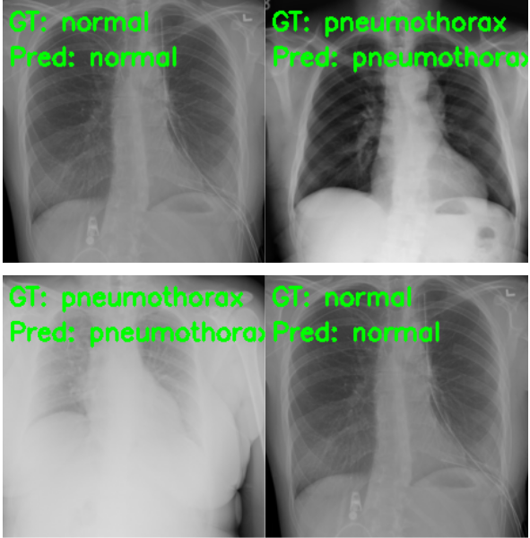
The results are great compared to what we had previously. Out of the 50 Pneumothorax cases, the model predicted 45 correctly and 5 as normal. But the most astonishing result is with the negative (normal) cases. This time, out of 50 normal images, 49 are predicted correctly, and only 1 is predicted incorrectly, whereas in the previous case none of the normal images were predicted correctly. And finally, let’s take a look at a few of the test predictions which were saved to disk.
Summary and Conclusion
In this tutorial, we carried forward the Pneumothorax binary classification problem using PyTorch by oversampling the negative classes. In our attempt to improve the accuracy and F1-score of the model, we applied augmentations to increase the dataset size manually and trained the model again. The model surely performed much better than the previous case. I hope that you learned something new in this tutorial.
If you have any doubts, thoughts, or suggestions, please leave them in the comment section. I will surely address them.
You can contact me using the Contact section. You can also find me on LinkedIn, and X.
