Comparing Wide Residual Networks and Residual Networks in PyTorch

In this article, we will compare two closely related models in terms of their performance. We will compare Wide Residual Networks and Residual Networks in PyTorch. Basically, we will use two pre-trained models from PyTorch Hub and compare their evaluation accuracies.

This is going to be a very hands-on tutorial with the inferencing of neural networks only. We will cover minimal theory in this tutorial and there is a reason for that as well.

So, what are we going to cover in this tutorial?

• A very short theory about Wide Residual Networks.
• Evaluation performance of Wide ResNet50_2 from PyTorch Hub.
• Evaluation Performance of ResNet152 from PyTorch Hub.

Wide Residual Networks

Let’s start with knowing about Wide Residual Networks a bit. We will cover very minimal things about Wide Residual Networks in this section. We will cover the release of the paper in short, why they are called so, and what are their advantages over standard Residual Networks.

The reason for the theory section being minimal is that we are going to cover Wide Residual Networks in much more detail in future tutorials. This includes the paper explanation as well as training them on common benchmark datasets like CIFAR10 and MNIST.

But in this tutorial, we will solely focus on the comparison between Wide Residual Networks and Residual Networks in PyTorch.

Wide Residual Networks

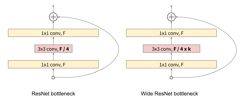
Wide Residual Networks or Wide ResNets or WRNs (as they are called for short) are a variant of Residual Networks (ResNets).

Wide ResNets were first introduced in the year 2016 by Sergey Zagoruyko and Nikos Komodakis. They tried to introduce a new variant of the standard ResNets and came up with Wide ResNets. So, instead of making the models deeper and thinner like the standard ResNets, they made the networks shallower and wider.

According to the authors, following are some of the important advantages of Wide Residual Networks.

• Wide Residual Networks have 50 times fewer layers and are 2 times faster.
• Their 16-layer wide network has the same accuracy as a 1000-layer thin neural network.
• Wide ResNets are faster to train. Meaning, they converge to the optimal solution much faster than standard ResNets.

Now, the above are some of the advantages of Wide Residual Networks. We will not be going any deeper than this in this tutorial. They require their own in-depth articles which we will cover in the near future. If you want to learn more, you can surely go through the paper here.

Let’s move on to the practical side of comparing Wide Residual Networks and Residual Networks in PyTorch.

Directory Structure

The following is the directory that we will be following through this tutorial.

│   evaluate.py
│   resnet.py
│   run.sh
│   wide_resnet.py
│
├───input
│       imagenet_classes.txt
│       image_1.png
│       image_2.jpg

• Directly inside the project directory, we have three Python scripts and one shell script. We will get into the content of these a bit later as we begin to write the code.
• The input folder contains two images. image_1.png is of a car and image_2.jpg is that of a TV monitor. These images are taken from Pixabay. So, they are completely free to use.

You can download the source code along with the input data for this tutorial by just clicking the button below.

The above files also contain an imagenet_classes.txt file which contains the 1000 ImageNet classes that we will need. We will use this file to map the output indices from the model to the names in the text file. Be sure to take a look at the file before you move ahead.

Now, just to have an idea of what are the two images inside the input folder, let’s take a look at them.

If you wish, you are free to use your own images for inferencing as well.

PyTorch Version

For this post, I have used PyTorch version 1.7.1 and Torchvision version 0.8.2. I recommend using these versions so that you have complete access to all the updated models while using Torch Hub.

Now, we are all set to start coding for comparison of Wide Residual Networks and Residual Networks in PyTorch.

Comparison of Wide Residual Networks and Residual Networks in PyTorch

From this section onward, we will start coding our way through this tutorial. We have thee Python scripts and one shell script. We will start with the evaluate.py Python script as that contains the most important code for this tutorial.

Write the Evaluation Code

As we will be comparing two different neural networks in this tutorial, most of the evaluation code is going to remain the same. This repetitive code will go into the evaluate.py Python file.

So, let’s start with importing the modules for this file.

import torch
import time

from torchvision import transforms
from PIL import Image

We are importing torch for PyTorch functionalities. We will use transforms for transforming the image and converting it to a tensor. Using Image, we will read the input image.

The Image Transforms

We will use very simple transforms as we are only carrying out the inference part. The following code block defines the tfms() function.

# define the image transforms for inference ...
# ... resize, convert to tensors, and normalize using imagenet stats
def tfms():
    transform = transforms.Compose([
        transforms.Resize((224, 224)),
        transforms.ToTensor(),
        transforms.Normalize(
            mean=[0.485, 0.456, 0.406],
            std=[0.229, 0.224, 0.225]
        )
    ])
    return transform

We will be resizing the image to the standard 224×224 dimensions for inference. Then we are converting the image to tensors and applying the normalization by using the ImageNet stats.

The Evaluation Function

We will write a simple function for evaluation that will carry out the whole process of evaluation. The following are the steps.

• Read the image from disk.
• Apply the transforms.
• Forward pass the input tensor through the model.
• Get the probabilities and map the outputs to the ImageNet classes.
• Print the top 5 probability outputs of the model.

The following is the eval() function.

def eval(model, device, image_path):
    # load the image
    image = Image.open(image_path).convert('RGB')
    # transform to convert to tensor
    transform = tfms()
    input_tensor = transform(image)
    # add batch dimension and load on to device
    input_tensor = input_tensor.unsqueeze(0).to(device)

    # forward pass the model through the model
    start = time.time()
    with torch.no_grad():
        output = model(input_tensor)
    end = time.time()
    print(f"Took {(end-start):.3f} seconds for forward pass...")

    # `output[0]` contains all the probabilities woth a dimension of 1000
    # this 1000 corresponds to 1000 ImageNet classes
    # the next line gets the softmax probabilities
    probs = torch.nn.functional.softmax(output[0], dim=0) 

    # load and read the imagenet classes file
    with open('input/imagenet_classes.txt', 'r') as f:
        # a list containing all the classes
        classes = [line.strip() for line in f.readlines()]

    # top 'k' class predictions of the image, 
    # ... you can choose k to be any number (e.g. top 3 or top 5)...
    # ... we are taking top 5 predictions
    k = 5
    topk_prob, topk_cat = torch.topk(probs, k)
    for i in range(topk_prob.size(0)):
        print(f"{classes[topk_cat[i]]} ---> {topk_prob[i].item():.3f}")

As we discussed, first, we are loading the image and applying the transforms from lines 19 to 23. We are also adding an extra batch dimension at line 25.

Starting from line 28, we are capturing the start time, then forward passing the image tensor through the neural network model, and then capturing the end time. The difference between the end and start time will give us an idea of how long it takes for one forward pass through the model.

Line 37 converts the output from the neural network model to softmax probabilities. These are 1000 probabilities in total which correspond to the 1000 classes from ImageNet.

Then we read the imagenet_classes.txt from disk and store all the classes in a classes list. Finally, starting from line 47, we get the top 5 probability values and their corresponding category id. We map this category id to the element in the classes list and print them along with the corresponding probability score. If you wish you can change the value of k to get that number of top probability scores and class labels.

This is all we need for the evaluation code.

Prepare the Wide ResNet Model

Now, we will write the code to prepare the Wide ResNet model.

Specifically, we will load the Wide ResNet50_2 model from PyTorch Hub. The name indicates that the model has a depth of 50 and a width of 2. What this depth and width mean, we will get into the details in future tutorials. For now, if you want to get some more details you can look at page 11 of the paper.

So, this code will go into the wide_resnet.py Python script.

import torch
import argparse

from evaluate import eval

# construct the argument parser
parser = argparse.ArgumentParser()
parser.add_argument('-i', '--input', help='path to input data', required=True)
args = vars(parser.parse_args())

# define the computation device 
device = torch.device('cuda:0' if torch.cuda.is_available() else 'cpu')

In the above code, we are importing the required modules and constructing the argument parser for the path to the input image. We are also defining the computation device for the model and image tensor. Note that we are importing our own evaluate module as well.

The next block of code loads the Wide ResNet model from PyTorch Hub.

model_name = 'wide_resnet50_2'
print(model_name)
# load the model from PyTorch Hub
model = torch.hub.load('pytorch/vision:v0.8.1', model_name,
                        pretrained=True)
# put the model into evaluation mode and load on to the computation device
model.eval().to(device)
# total parameters in the model
total_params = sum(p.numel() for p in model.parameters())
print(f"[INFO]: {total_params:,} total parameters.")

eval(model, device, args['input'])
print('-' * 50)

We are printing the model name so that we can know which model is executing currently. We will get to see why this is important just a bit later. Then we are loading the Wide ResNet50_2 from PyTorch Hub with all the pre-trained weights.

At line 19, we are putting the model into evaluation mode and loading it onto the computation device. We are also printing the number of parameters in the model. This will provide us with some useful information.

Finally, we are executing the eval() function by passing the model, the computation device, and the image path as parameters. The rest of the evaluation process will be handled by the evaluate module.

This completes the code for preparing the Wide ResNet model and using it for inferencing.

Prepare the ResNet152 Model

For the simple Residual network, we will be using the ResNet152 model from PyTorch Hub. The reason being, it is very similar in terms of number of parameters and top-1% error to the Wide ResNet50_2 model. But according to the paper, the Wide ResNet50_2 model is slightly better than that. So, let’s see if it really holds up.

The code for preparing the ResNet152 model is going to be almost exactly same as it was for Wide ResNet50_2. We only need to load a different model.

This code will go into the resnet.py Python script.

import torch
import argparse

from evaluate import eval

# construct the argument parser
parser = argparse.ArgumentParser()
parser.add_argument('-i', '--input', help='path to input data', required=True)
args = vars(parser.parse_args())

# define the computation device 
device = torch.device('cuda:0' if torch.cuda.is_available() else 'cpu')

model_name = 'resnet152'
print(model_name)
# load the model from PyTorch Hub
model = torch.hub.load('pytorch/vision:v0.8.1', model_name,
                        pretrained=True)
# put the model into evaluation mode and load on to the computation device
model.eval().to(device)
# total parameters in the model
total_params = sum(p.numel() for p in model.parameters())
print(f"[INFO]: {total_params:,} total parameters.")

eval(model, device, args['input'])
print('-' * 50)

At line 17, we are loading the ResNet152 model and everything else is same as the Wide ResNet50_2 code.

The Shell Script to Run all The Code Files

Remember that we have a shell script as well. This script will not contain anything special or difficult. It will just contain the execution commands for the Python scripts with the correct path flags for the argument parser. This will ensure that we only have to execute one file and everything else will run automatically.

Let’s write the code in run.sh file.

python wide_resnet.py --input input/image_1.png
python resnet.py --input input/image_1.png

python wide_resnet.py --input input/image_2.jpg
python resnet.py --input input/image_2.jpg

So, the first two lines execute the inference for Wide ResNet50_2 and ResNet152 model for the same image. image_1.png is that of a car.

The 3rd and 4th lines execute the Wide ResNet50_2 and ResNet152 inference for the second image, that is that of a TV monitor.

After executing this shell script, we will have 4 different outputs with confidence scores and time taken for the forward pass.

Execute run.sh for Comparing Wide Residual Networks and Residual Networks in PyTorch

Let execute the run.sh script and see what outputs we are getting.

Open up your command line/terminal inside the project directory and execute the following command.

sh run.sh

You should see output similar to the following.

wide_resnet50_2
[INFO]: 68,883,240 total parameters.
Took 1.009 seconds for forward pass...
convertible ---> 0.878
car wheel ---> 0.064
sports car ---> 0.026
grille ---> 0.011
beach wagon ---> 0.007
--------------------------------------------------
resnet152
[INFO]: 60,192,808 total parameters.
Took 1.025 seconds for forward pass...
convertible ---> 0.755
beach wagon ---> 0.091
grille ---> 0.074
car wheel ---> 0.054
pickup ---> 0.010
--------------------------------------------------
wide_resnet50_2
[INFO]: 68,883,240 total parameters.
Took 1.037 seconds for forward pass...
monitor ---> 0.799
screen ---> 0.160
television ---> 0.010
desktop computer ---> 0.008
web site ---> 0.005
--------------------------------------------------
resnet152
[INFO]: 60,192,808 total parameters.
Took 1.033 seconds for forward pass...
monitor ---> 0.406
screen ---> 0.134
notebook ---> 0.109
desktop computer ---> 0.091
iPod ---> 0.063
--------------------------------------------------

Okay, we have the results. We can clearly see which inference was using Wide ResNet50_2 and which was using ResNet152.

The first two inference results are for the car image. The first thing we can notice is that the Wide ResNet50_2 model is just a bit faster than the ResNet152 model. And this is in spite of the fact that it has 8 million more parameters than ResNet152. Coming to the probability scores, let’s focus on the first one of the top 5 results. Both the models are classifying it as a convertible (a type of car). But the Wide Resnet50_2 model is classifying it with a probability of 0.878. Whereas, the ResNet152 model is classifying it with a probability of 0.755. Obviously, the Wide ResNet model wins in this case.

Coming to the second image (TV monitor), both models are classifying it as monitor with the highest probability. But again the Wide ResNet wins with a probability of 0.799 compared to 0.406 of ResNet152.

From the above results, it is clear that the Wide ResNet model is faster and performs better as well.

Going Further from Here…

You can also try this script with different images and share your results in the comment section. We did not cover the extensive theory of Wide ResNets in this tutorial. We will do that in upcoming posts. And we will also implement the training of Wide ResNets.

Stay tuned for that.

Summary and Conclusion

In this tutorial, we did a comparison of Wide Residual Networks and Residual Networks in PyTorch. We observed that Wide ResNets perform better than standard ResNets in terms of speed and classification scores. I hope that you learned something new from this tutorial.

If you have any doubts, thoughts, or suggestions, then please leave them in the comment section. I will surely address them.

You can contact me using the Contact section. You can also find me on LinkedIn, and Twitter.