Traffic Sign Recognition using Custom Image Classification Model in PyTorch

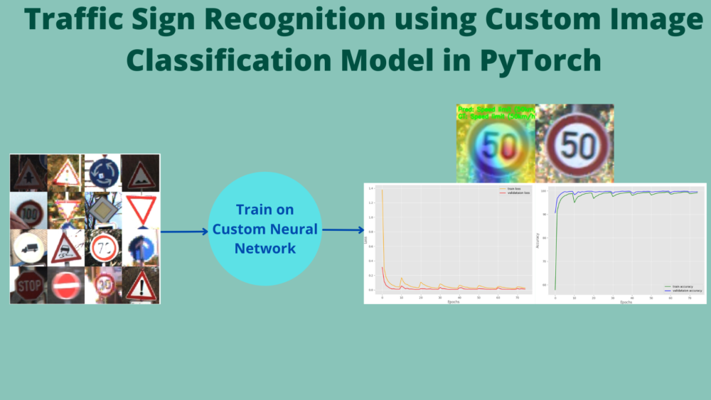
In this tutorial, we will be carrying out traffic sign recognition using a custom image classification model in PyTorch. Specifically, we will build and train a tiny custom Residual Neural Network on the German Traffic Sign Recognition Benchmark dataset.

This post is part of the traffic sign recognition and detection series.

• Traffic Sign Recognition using PyTorch and Deep Learning.
• Traffic Sign Detection using PyTorch and Pretrained Faster RCNN Model.
• Using Any Torchvision Pretrained Model as Backbone for PyTorch Faster RCNN
• Traffic Sign Recognition using Custom Image Classification Model in PyTorch

There are a lot of PyTorch pretrained models available via Torchvision. And we have been leveraging those models for traffic sign recognition and detection. Till now we have done the following things in this series.

• We started by using a MobileNetV3 pretrained classification model and fine-tuning it on the GTSRB dataset.
• Then we moved on to detection. We used Faster RCNN models pretrained on the COCO dataset and trained it on the GTSDB dataset.
• We also got to know how to use different Torchvision pretrained classification models as backbones for the Faster RCNN head.

Using PyTorch as the deep learning framework of choice made all of this easier for us. But the story does not end here. There are a few more experiments in this series that we carry on further.

• One is creating our custom image classification (recognition) model and training on the GTSRB dataset.
• Another, using the same recognition model as the backbone for the Faster RCNN head. This we will do in the next post.

For this post, specifically, we will focus on creating our custom Residual Neural Network. Then we will carry out traffic sign recognition using a custom image classification model in PyTorch on the GTSRB dataset. Although a lot of things will remain the same, a few things will change in the classification pipeline. And anyhow, this will be a good learning point for how a model behaves when training on a large dataset from scratch.

Points To Cover in This Post

We will cover the following points in this post:

• We will start with a short discussion of the GTSRB (German Traffic Sign Recognition Benchmark) dataset. Along with that, we will also check out a few images from the dataset.
• As a lot of things are already covered in the first GTSRB recognition post in this series, we will only focus on the new things. The coding section includes knowing about the custom image classification model that we will use.
• After training, we will carry out inference on the test set and also visualize the class activation maps. This section will also cover the accuracy that we get on the test set.
• We will end the post with some of the advantages and disadvantages that we get while using a custom model from scratch.

This tutorial will form the basis of a few more tutorials along the way. Of course, this is the basis for the very next one where we will use this custom residual neural network as the backbone for the PyTorch Faster RCNN model. Along with that, in the near future, we will also learn about the practical aspects of ResNets as well as write ResNets from scratch.

The GTSRB Dataset

We have already discussed the GTSRB dataset in detail in the first post of this series. So, we will cover it very briefly here.

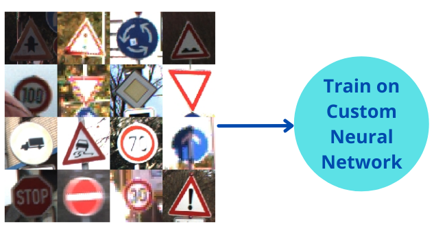
In short, the dataset contains images of German traffic signs in real-life settings. It contains more than 50000 images distributed across 43 classes. The following figure shows some of the images from the dataset.

If you wish to learn more about the dataset, please visit this post.

If you are directly covering this tutorial, then you may need to download the GTSRB dataset files. This is needed if you wish to train the model yourself.

You can either download the files via this webpage. Or you can click on the following to access the direct download links.

• GTSRB_Final_Training_Images.zip
• GTSRB_Final_Test_Images.zip
• GTSRB_Final_Test_GT.zip

In the next section, we will discuss the directory structure to know where to extract the above zip files.

Directory Structure

The directory structure for this tutorial/project will be exactly similar to what was in the case of the first tutorial in the series. Let’s take a look at that.

├── input
│   ├── GTSRB_Final_Test_GT
│   │   └── GT-final_test.csv
│   ├── GTSRB_Final_Test_Images
│   │   └── GTSRB
│   │       ├── Final_Test
│   │       │   └── Images [12631 entries exceeds filelimit, not opening dir]
│   │       └── Readme-Images-Final-test.txt
│   ├── GTSRB_Final_Training_Images
│   │   └── GTSRB
│   │       ├── Final_Training
│   │       │   └── Images
│   │       │       ├── 00000 [211 entries exceeds filelimit, not opening dir]
│   │       │       ├── 00001 [2221 entries exceeds filelimit, not opening dir]
                    ...
│   │       │       ├── 00040 [361 entries exceeds filelimit, not opening dir]
│   │       │       ├── 00041 [241 entries exceeds filelimit, not opening dir]
│   │       │       └── 00042 [241 entries exceeds filelimit, not opening dir]
│   │       └── Readme-Images.txt
│   ├── README.txt
│   └── signnames.csv
├── outputs
│   ├── test_results [12630 entries exceeds filelimit, not opening dir]
│   ├── accuracy.png
│   ├── loss.png
│   └── model.pth
└── src
    ├── cam.py
    ├── datasets.py
    ├── model.py
    ├── train.py
    └── utils.py

There are no changes in the directory structure apart from the content in some of the Python files. We will discuss these changes in the respective coding section.

To get an idea of the content, here is a short overview of the directory structure.

• The input directory contains the three dataset folders after extracting them along with a CSV file holding the ground truth for the test images.
• The outputs directory will hold the outputs generated from training and inference. The final inference results on the test set will be saved in the test_results subdirectory.
• Finally, the src directory contains the Python files.

This is all we need to know about the directory structure.

Be sure to download the zip file for this tutorial to get access to the trained model and the Python source code.

Libraries and Frameworks

The dependencies of libraries and frameworks remain the same throughout the series. We will use PyTorch 1.10.0 and Albumentations 1.1.0.

• Install the latest version of PyTorch from here.
• Install the latest version of Albumentations from here.

Traffic Sign Recognition using Custom Image Classification Model in PyTorch

From this section, we will begin the discussion of the important Python files. A lot of the Python code files remain the same. The files that we will discuss are:

• The model.py file which contains the new tiny custom residual neural network model.
• We will also discuss the changes in the cam.py briefly before carrying out the inference.

Let’s get on to the discussion of the custom residual neural network.

The Custom Residual Neural Network

Before we move on to the custom residual neural network that we use here, let’s point out a few things:

• We will not go into the very details of building a custom residual neural network here. That requires it’s own post to do proper justice.
• We will just go through the building blocks of the model in this section.
• There are going to be proper posts in the near future building and explaining official ResNets and custom ResNets from scratch. We will get into the details there for sure.

For now, if you want to know more about ResNets, these posts may help you.

• Residual Neural Networks – ResNets: Paper Explanation
• Wide Residual Neural Networks – WRNs: Paper Explanation

Here, we will only cover the important aspects of building a custom model for traffic sign recognition using PyTorch.

The model code is present in the model.py file in the src directory.

The following are the two import statements that we need to create the custom residual neural network.

from torch import nn
from torch.nn import functional as F

The neural network that we will be building here is a very simple one. The most important rule that it follows in its residual block is the following:

$$
y = {F}(x) + x
$$

The Residual Block

In the residual block of the network, we add the direct inputs of the network to the outputs that have passed through a few layers. Let’s take a look at the code of the Residual block which will make things clearer.

class ResidualBlock(nn.Module):
    """
    Creates the Residual block of ResNet.
    """
    def __init__(
        self, in_channels, out_channels, use_1x1conv=True, strides=1
    ):
        super().__init__()
        self.conv1 = nn.Conv2d(in_channels, out_channels,
                               kernel_size=3, padding=1, stride=strides)
        self.conv2 = nn.Conv2d(out_channels, out_channels,
                               kernel_size=3, padding=1)
        if use_1x1conv:
            self.conv3 = nn.Conv2d(in_channels, out_channels,
                                   kernel_size=1, stride=strides)
        else:
            self.conv3 = None
        self.bn1 = nn.BatchNorm2d(out_channels)
        self.bn2 = nn.BatchNorm2d(out_channels)

    def forward(self, x):
        inputs = x
        x = F.relu(self.bn1(self.conv1(x)))
        x = self.bn2(self.conv2(x))
        if self.conv3:
            inputs = self.conv3(inputs)
        x += inputs
        return F.relu(x)

The above code block defines the entire residual block of a residual neural network. In the __init__() method, we define the 2D convolutional layers with respective input and output channels. We are also checking whether to use 1×1 2D convolution or not depending on the input parameters.

The forward() method, first makes a copy of the actual input, that is x, and stores it in inputs. We can see that on line 29, we add the original inputs to the output that has been obtained from all the previous layers.

Create Instances of Residual Block

Next, we have the create_resnet_block() function that creates the above residual blocks depending on the number of blocks we want to create.

def create_resnet_block(
    input_channels,
    output_channels, 
    num_residuals,
):
        resnet_block = []
        for i in range(num_residuals):
            if i == 0:
                resnet_block.append(ResidualBlock(input_channels, output_channels,
                                    use_1x1conv=True, strides=2))
            else:
                resnet_block.append(ResidualBlock(output_channels, output_channels))
        return resnet_block 

We are passing the number of input_channels, output_channels, and num_residuals that we want to create. According to this number, the instances of the ResidualBlock are created and appended to resnet_block.

The Final Model

Now, we have to write one custom model class that will combine the above two and provide us with the final custom ResNet model.

class CustomResNet(nn.Module):
    def __init__(self, num_classes=10):
        super().__init__()
        self.block1 = nn.Sequential(
            nn.Conv2d(3, 16, kernel_size=7, stride=2, padding=3),
            nn.BatchNorm2d(16), 
            nn.ReLU(),
            nn.MaxPool2d(kernel_size=3, stride=2, padding=1)
        )
        self.block2 = nn.Sequential(*create_resnet_block(16, 32, 2))
        self.block3 = nn.Sequential(*create_resnet_block(32, 64, 2))
        self.block4 = nn.Sequential(*create_resnet_block(64, 128, 2))
        self.block5 = nn.Sequential(*create_resnet_block(128, 256, 2))

        self.linear = nn.Linear(256, num_classes)

    def forward(self, x):
        x = self.block1(x)
        x = self.block2(x)
        x = self.block3(x)
        x = self.block4(x)
        x = self.block5(x)
        bs, _, _, _ = x.shape
        x = F.adaptive_avg_pool2d(x, 1).reshape(bs, -1)
        x = self.linear(x)
        return x 

As you can see, in the __init__() method we define all the residual blocks by calling the create_resnet_block function. Only for block1, we define the layers manually. But they are all Sequential layers that can be easily combined together. Also, you can observe that we are using very small values for output channels. This is because we want to keep our custom neural network pretty small in terms of parameters. This will help us achieve a very high speed for traffic sign recognition using the custom model in PyTorch.

In the forward() method, we simply pass the data through all the layers and return the output.

If you want to get a proper idea of the network that we are building here, the following blocks shows the output from print(model).

CustomResNet(
  (block1): Sequential(
    (0): Conv2d(3, 16, kernel_size=(7, 7), stride=(2, 2), padding=(3, 3))
    (1): BatchNorm2d(16, eps=1e-05, momentum=0.1, affine=True, track_running_stats=True)
    (2): ReLU()
    (3): MaxPool2d(kernel_size=3, stride=2, padding=1, dilation=1, ceil_mode=False)
  )
  (block2): Sequential(
    (0): ResidualBlock(
      (conv1): Conv2d(16, 32, kernel_size=(3, 3), stride=(2, 2), padding=(1, 1))
      (conv2): Conv2d(32, 32, kernel_size=(3, 3), stride=(1, 1), padding=(1, 1))
      (conv3): Conv2d(16, 32, kernel_size=(1, 1), stride=(2, 2))
      (bn1): BatchNorm2d(32, eps=1e-05, momentum=0.1, affine=True, track_running_stats=True)
      (bn2): BatchNorm2d(32, eps=1e-05, momentum=0.1, affine=True, track_running_stats=True)
    )
    (1): ResidualBlock(
      (conv1): Conv2d(32, 32, kernel_size=(3, 3), stride=(1, 1), padding=(1, 1))
      (conv2): Conv2d(32, 32, kernel_size=(3, 3), stride=(1, 1), padding=(1, 1))
      (conv3): Conv2d(32, 32, kernel_size=(1, 1), stride=(1, 1))
      (bn1): BatchNorm2d(32, eps=1e-05, momentum=0.1, affine=True, track_running_stats=True)
      (bn2): BatchNorm2d(32, eps=1e-05, momentum=0.1, affine=True, track_running_stats=True)
    )
  )
  (block3): Sequential(
    (0): ResidualBlock(
      (conv1): Conv2d(32, 64, kernel_size=(3, 3), stride=(2, 2), padding=(1, 1))
      (conv2): Conv2d(64, 64, kernel_size=(3, 3), stride=(1, 1), padding=(1, 1))
      (conv3): Conv2d(32, 64, kernel_size=(1, 1), stride=(2, 2))
      (bn1): BatchNorm2d(64, eps=1e-05, momentum=0.1, affine=True, track_running_stats=True)
      (bn2): BatchNorm2d(64, eps=1e-05, momentum=0.1, affine=True, track_running_stats=True)
    )
    (1): ResidualBlock(
      (conv1): Conv2d(64, 64, kernel_size=(3, 3), stride=(1, 1), padding=(1, 1))
      (conv2): Conv2d(64, 64, kernel_size=(3, 3), stride=(1, 1), padding=(1, 1))
      (conv3): Conv2d(64, 64, kernel_size=(1, 1), stride=(1, 1))
      (bn1): BatchNorm2d(64, eps=1e-05, momentum=0.1, affine=True, track_running_stats=True)
      (bn2): BatchNorm2d(64, eps=1e-05, momentum=0.1, affine=True, track_running_stats=True)
    )
  )
  (block4): Sequential(
    (0): ResidualBlock(
      (conv1): Conv2d(64, 128, kernel_size=(3, 3), stride=(2, 2), padding=(1, 1))
      (conv2): Conv2d(128, 128, kernel_size=(3, 3), stride=(1, 1), padding=(1, 1))
      (conv3): Conv2d(64, 128, kernel_size=(1, 1), stride=(2, 2))
      (bn1): BatchNorm2d(128, eps=1e-05, momentum=0.1, affine=True, track_running_stats=True)
      (bn2): BatchNorm2d(128, eps=1e-05, momentum=0.1, affine=True, track_running_stats=True)
    )
    (1): ResidualBlock(
      (conv1): Conv2d(128, 128, kernel_size=(3, 3), stride=(1, 1), padding=(1, 1))
      (conv2): Conv2d(128, 128, kernel_size=(3, 3), stride=(1, 1), padding=(1, 1))
      (conv3): Conv2d(128, 128, kernel_size=(1, 1), stride=(1, 1))
      (bn1): BatchNorm2d(128, eps=1e-05, momentum=0.1, affine=True, track_running_stats=True)
      (bn2): BatchNorm2d(128, eps=1e-05, momentum=0.1, affine=True, track_running_stats=True)
    )
  )
  (block5): Sequential(
    (0): ResidualBlock(
      (conv1): Conv2d(128, 256, kernel_size=(3, 3), stride=(2, 2), padding=(1, 1))
      (conv2): Conv2d(256, 256, kernel_size=(3, 3), stride=(1, 1), padding=(1, 1))
      (conv3): Conv2d(128, 256, kernel_size=(1, 1), stride=(2, 2))
      (bn1): BatchNorm2d(256, eps=1e-05, momentum=0.1, affine=True, track_running_stats=True)
      (bn2): BatchNorm2d(256, eps=1e-05, momentum=0.1, affine=True, track_running_stats=True)
    )
    (1): ResidualBlock(
      (conv1): Conv2d(256, 256, kernel_size=(3, 3), stride=(1, 1), padding=(1, 1))
      (conv2): Conv2d(256, 256, kernel_size=(3, 3), stride=(1, 1), padding=(1, 1))
      (conv3): Conv2d(256, 256, kernel_size=(1, 1), stride=(1, 1))
      (bn1): BatchNorm2d(256, eps=1e-05, momentum=0.1, affine=True, track_running_stats=True)
      (bn2): BatchNorm2d(256, eps=1e-05, momentum=0.1, affine=True, track_running_stats=True)
    )
  )
  (linear): Linear(in_features=256, out_features=43, bias=True)
)
2,892,491 total parameters.
2,892,491 training parameters.

The model contains just below 2.9 million parameters. Although this is pretty small, hopefully, the residual blocks will help us achieve very good results.

Training the Custom ResNet on the Traffic Sign Dataset

Note: All training and inference experiments were carried out on a machine with an i7 10th gen CPU, 32GB RAM, and 10GB RTX 3080 GPU. Your training time may vary according to the hardware.

All the other Python files remain the same. We can directly start training and check out the results.

Open your terminal/command line and execute the following command within the src directory.

python train.py --epochs 75

We are training the model for 75 epochs. The learning is the default, 0.001 as we are training the model from scratch here. But just as the first tutorial in the series, we use the CosineAnnealingWarmRestarts scheduler here with a restart period of 10 epochs.

Results for Traffic Sign Recognition using Custom Model in PyTorch

The following block shows the terminal output in a truncated format.

[INFO]: Number of training images: 35289
[INFO]: Number of validation images: 3920
[INFO]: Class names: ['00000', '00001', '00002', '00003', '00004', '00005', '00006', '00007', '00008', '00009', '00010', '00011', '00012', '00013', '00014', '00015', '00016', '00017', '00018', '00019', '00020', '00021', '00022', '00023', '00024', '00025', '00026', '00027', '00028', '00029', '00030', '00031', '00032', '00033', '00034', '00035', '00036', '00037', '00038', '00039', '00040', '00041', '00042']

Computation device: cuda
Learning rate: 0.001
Epochs to train for: 75

2,892,491 total parameters.
2,892,491 training parameters.
Epoch     0: adjusting learning rate of group 0 to 1.0000e-03.
[INFO]: Epoch 1 of 75
Training
100%|████████████████████████████████████████████████████████████████████████████████████████████████████████████████████████████████████████████████████████████████████████████| 276/276 [00:15<00:00, 17.84it/s]
Validation
100%|██████████████████████████████████████████████████████████████████████████████████████████████████████████████████████████████████████████████████████████████████████████████| 31/31 [00:01<00:00, 26.69it/s]


Accuracy of class 00000: 72.0
Accuracy of class 00001: 94.23868312757202
...
[INFO]: Epoch 75 of 75
Training
100%|████████████████████████████████████████████████████████████████████████████████████████████████████████████████████████████████████████████████████████████████████████████| 276/276 [00:14<00:00, 19.53it/s]
Validation
100%|██████████████████████████████████████████████████████████████████████████████████████████████████████████████████████████████████████████████████████████████████████████████| 31/31 [00:01<00:00, 28.55it/s]


Accuracy of class 00000: 100.0
Accuracy of class 00001: 99.58847736625515
Accuracy of class 00002: 99.55555555555556
Accuracy of class 00003: 99.34210526315789
Accuracy of class 00004: 100.0
Accuracy of class 00005: 99.0
Accuracy of class 00006: 100.0
Accuracy of class 00007: 99.37106918238993
Accuracy of class 00008: 99.31506849315069
Accuracy of class 00009: 99.29577464788733
Accuracy of class 00010: 100.0
Accuracy of class 00011: 100.0
Accuracy of class 00012: 100.0
Accuracy of class 00013: 100.0
Accuracy of class 00014: 100.0
Accuracy of class 00015: 100.0
Accuracy of class 00016: 100.0
Accuracy of class 00017: 100.0
Accuracy of class 00018: 100.0
Accuracy of class 00019: 100.0
Accuracy of class 00020: 97.22222222222223
Accuracy of class 00021: 100.0
Accuracy of class 00022: 100.0
Accuracy of class 00023: 100.0
Accuracy of class 00024: 100.0
Accuracy of class 00025: 100.0
Accuracy of class 00026: 100.0
Accuracy of class 00027: 100.0
Accuracy of class 00028: 100.0
Accuracy of class 00029: 100.0
Accuracy of class 00030: 94.82758620689656
Accuracy of class 00031: 100.0
Accuracy of class 00032: 100.0
Accuracy of class 00033: 100.0
Accuracy of class 00034: 100.0
Accuracy of class 00035: 100.0
Accuracy of class 00036: 100.0
Accuracy of class 00037: 100.0
Accuracy of class 00038: 99.42857142857143
Accuracy of class 00039: 100.0
Accuracy of class 00040: 100.0
Accuracy of class 00041: 100.0
Accuracy of class 00042: 100.0


Training loss: 0.027, training acc: 99.235
Validation loss: 0.011, validation acc: 99.668
--------------------------------------------------
TRAINING COMPLETE

If you check the datasets.py file, you may note that we are using pretty heavy augmentation for the training set. For that reason, the training loss and accuracy are slightly worse compared to the validation ones.

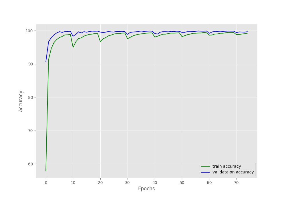
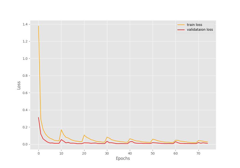
The rise and dips in the loss and accuracy plots respectively are the epochs where the learning rate became 0 and then again rose to the original value.

This time the results are slightly lower as we are training a model from scratch. In the first post of the series, the model gave 100% validation accuracy and 0 validation loss. Then again, that was a pretrained MobileNetV3 Large model with over 4 million parameters. These results here with custom model training from scratch look pretty good as well.

Inference and Visualizing Class Activation Maps (CAM)

We will use the cam.py script to carry out the final inference on the test images and visualize the class activation maps as well. There is just a small change in the script this time. As we are using a different model this time, we need to register the forward hook on block5 of the model. Essentially, the code for hooking the feature extractor looks like this (lines 93 to 99 in cam.py).

# Hook the feature extractor.
# https://github.com/zhoubolei/CAM/blob/master/pytorch_CAM.py
features_blobs = []
def hook_feature(module, input, output):
    features_blobs.append(output.data.cpu().numpy())
model._modules.get('block5').register_forward_hook(hook_feature)
# Get the softmax weight.
params = list(model.parameters())
weight_softmax = np.squeeze(params[-2].data.cpu().numpy())

Line 6 in the above blocks shows that change. Apart from that everything remains the same and you can also find a brief description of the entire code in the first tutorial of the series.

Execute the script from the same src directory.

python cam.py 

The Inference and CAM Results

The outputs should be similar to the following.

Image: 1
Image: 2
...
Image: 12629
Image: 12630
Total number of test images: 12630
Total correct predictions: 12187
Accuracy: 96.492
Average FPS: 321.390

This time the accuracy is around 2% lower. This is still good keeping in mind how small our model is and we are training from scratch. And the small model is helping achieve a really high FPS of 321 compared to 178 FPS in the case of MobileNetV3 Large. This increase in FPS will also reciprocate when using the model as a backbone for the Faster RCNN detection head.

Now, let’s check out a few of the class activation map results.

In most instances, models seem to be focusing around the edges of the traffic signs which still seems pretty plausible. There are some cases though, where the model is at the surrounding areas as well but making the correct predictions.

Overall, the model seems to have learned the features of the dataset very well.

Advantages and Disadvantages

One of the major advantages was that we were able to build a pretty small model. But obviously, it did not perform just as well as an ImageNet pretrained model.

Summary and Conclusion

In this tutorial, we carried out traffic sign recognition training using a custom residual neural network model in PyTorch. Our model was small and simple, yet it learned the dataset pretty well and also gave more than 96% test accuracy. In the next tutorial, we will use the same model architecture as a backbone for PyTorch Faster RCNN. There, we will see what changes we have to make to the model to prepare it to be a suitable backbone. I hope that this tutorial was helpful for you.

If you have any doubts, thoughts, or suggestions, please leave them in the comment section. I will surely address them.

You can contact me using the Contact section. You can also find me on LinkedIn, and Twitter.