In the last post, we carried out traffic sign recognition on the GTSRB dataset. Here, in this post, we will take a step further. We will carry out traffic sign detection using PyTorch and pretrained Faster RCNN models.
From the last post, it was pretty clear that a complete traffic sign recognition system requires two components. The classification and detection of the traffic signs. In the real world, any autonomous vehicle, first detects where a traffic sign is (detection/localization) and applies recognition to it (image classification). Again, this post is not about replicating any component of autonomous driving. It is just about knowing the very basic procedures and concepts through a toy object detection project. But hopefully, it will turn out to be both fun and inspiring.
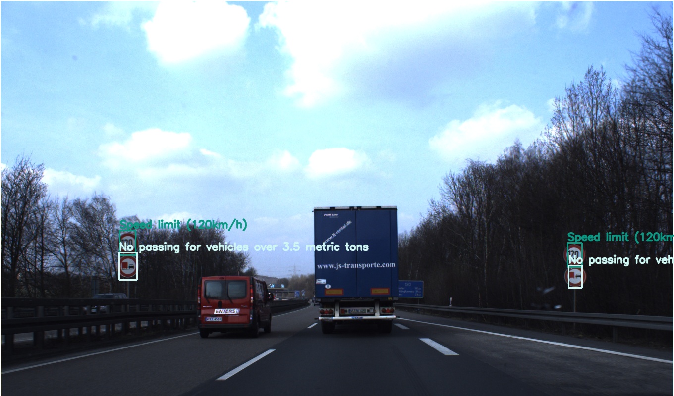
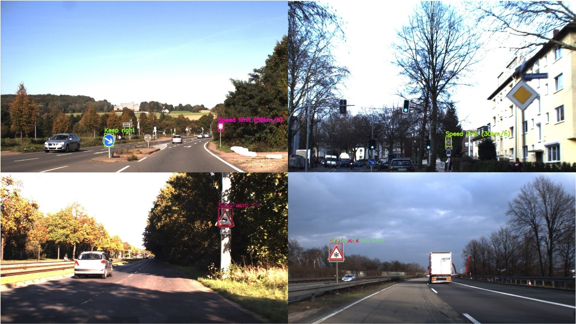
Figure 1. One of the inference results from traffic sign detection using PyTorch and Faster RCNN. We will train a model that is capable of such detections.
And obviously, for traffic sign detection using PyTorch, we will not be building anything from scratch. We will leverage existing pretrained models and utilities to create an end-to-end pipeline for traffic sign detection. In fact, we will try to keep it as modular as possible so that you can switch with any dataset in the future and just change the dataset path. Specifically, we will use the Faster RCNN model for detection here. We will fine-tune a pretrained MobileletNetV3 Large Faster RCNN model and check out the inference performance on both images and videos.
This is the second post in the traffic sign recognition and detection series.
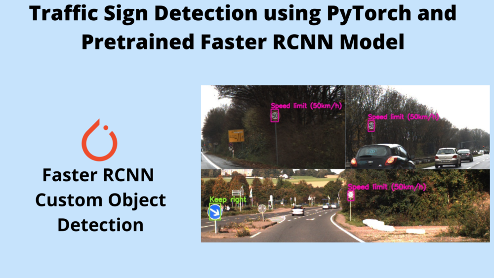
Traffic Sign Detection using PyTorch and Pretrained Faster RCNN Model
Topics to Cover
We will cover the following topics in this post:
We will start with the exploration of the dataset that we will use for traffic sign detection. This is the GTSDB dataset.
During the coding phase, we will focus on a few very important things. These inlcude:
The dataset preparation in the correct format. This is the step before creating the PyTorch dataset and PyTorch data loaders.
Then we will discuss the configuration Python file.
In regard to the training and inference dataset, we will mostly focus on the augmentations that we apply for object detection here.
Then we will discuss the training script in brief.
After the training completes, we will discuss the inference code. Then carry out inference on images and videos.
Finally, we will end the post by discussing some of the further steps that we can take to make this project even better.
The GTSDB Dataset
We will use the German Traffic Sign Detection Benchmark dataset for traffic sign detection using PyTorch and Faster RCNN in this post. This dataset was mainly created for researchers who wanted to take on the task of an image-based driver assistance system. Although a bit old, this dataset will perfectly fit our purpose of learning more about object detection and testing different Faster RCNN models on it.
This dataset is closely related to the German Traffic Sign Recognition Benchmark dataset. The GTSDB dataset contains the same classes as GTSRB. And it was also part of the IJCNN (International Joint Conference on Neural Networks) 2013.
The following are a few important details about the dataset:
It contains a total of 900 images. 600 of them are training images and 300 are for evaluation.
It contains 43 classes, out of which the following are a few:
You can easily explore all the images and classes after downloading the entire dataset.
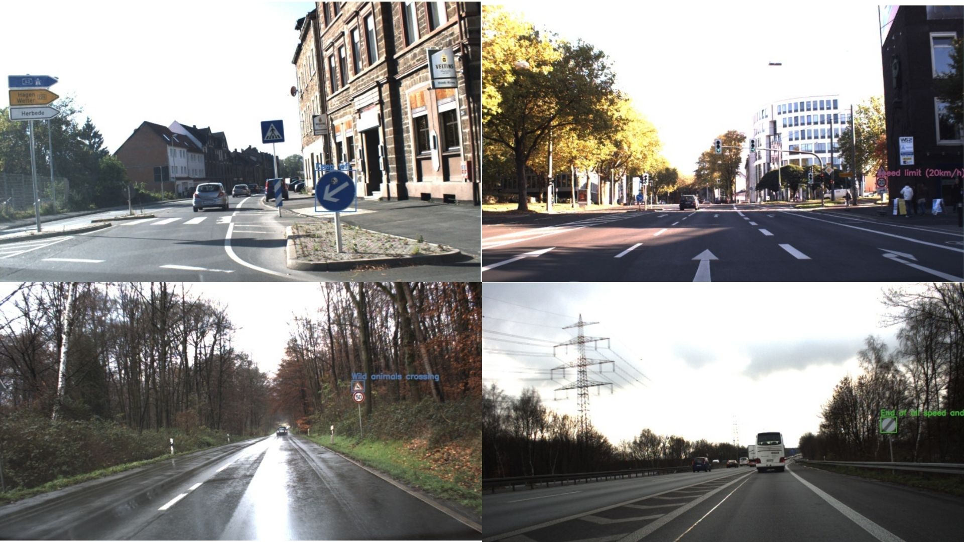
Also, to get a sense of the type of the objects and the classes, the following figure shows a few traffic signs along with the annotations.
Figure 2. Traffic sign images with ground truth annotations.
As we can see, some of the signs are pretty difficult to recognize as they are very small. Only a really good object detection model will be able to perform well on this dataset. In this post, we will check out the performance of two different Faster RCNN models. This will give us a good idea of what kind of detector is better suited for such a dataset.
Downloading the Dataset
There are a few mandatory dataset files that you need to download via this link. You need to download the TrainIJCNN2013.zip, TestIJCNN2013.zip, and gt.txt files. You can visit the link to download them or click on the following direct download links:
There are a few other files that we need but you will get direct access to them when downloading the zip file for this post. And we will also process and prepare the training and validation images out of the original images which are part of the coding section in this post.
The Original Dataset Structure
For now, let’s take a look at the original structure of the downloaded files. This is after extracting the downloaded zip files.
The TrainIJCNN2013 directory first contains the 43 class folders which contain a few sample images belonging to the respective classes. But all the images starting from 00000.ppm to 00599.ppm are present directly inside the TrainIJCNN2013. Along with that, it also contains gt.txt file which holds the ground truth annotations and classes in the following format:
All the attributes are separated by semi-colons. The first one is the image/file name and the next four are the bounding box coordinates in the x_min, y_min, x_max, and y_max format. In other words, they are the top-left and bottom-right coordinates of the traffic signs in a particular image. The final attribute is the class number. The ReadMe.txt file contains the mapping of the class number to the class names along with a few other information.
The TestIJCNN2013 directory directly contains the 300 test images without any ground truth information. This is because the test set results were meant to be submitted to the competition site for evaluation. But we will use these images for inference after training the model.
The Project Directory Structure
Now, let’s take a look at the entire directory structure for this post. This will give us a better idea on how to arrange each file and folder.
Okay! There are a lot of things to cover here and a few important ones too. So, let’s go through them.
We have already seen a lot of content in the input directory in the previous section. In short, it contains all the data related files and folders. The inference_data subdirectory contains the video file that we will use for inference. The classes_list.txt file contains all the class names in a text format for easier management of the all the class names. signnames.csv contains the class number and class name mappings in CSV format. We will generate the train_images, train_xmls, valid_images, valid_xmls, all_annots.csv, train.csv, and valid.csv through the data preparation scripts. That we will cover in the coding section.
The outputs and inference_outputs directories will contain the training and inference results respectively.
Now coming to the src directory. Mostly, we will cover all the content of this in the coding section. Still, just to have a brief idea, the following are the scripts and Python files we have:
The models subdirectory contains the code to load two different Faster RCNN models.
The torch_utils subdirectory contains the different utility scripts such as COCO mAP calculation scripts, training and validation fucntions (engine.py), and other helper functions (utils.py). Most of the code in this subdirectory has been borrowed from the original PyTorch detection repository and slightly modified according to our use case.
Other Python files directly in the src directory are custom written. These consist of training, inference, and data preparation scripts.
You will get access to all the code files, the trained model, outputs, and a few of the files in the input directory when downloading the zip file for this post.
Libraries and Frameworks
The two major libraries for this project are PyTorch and Albumentations. All the code has been developed using PyTorch 1.10.0 and Albumentations 1.1.0. Newer versions of these two libraries should not cause any issues as well.
Traffic Sign Detection using PyTorch and Pretrained Faster RCNN Model
Starting from this section, we will start discussing the coding part of the post. By now, you must have realized that there are a lot of Python files accompanying this post. You will surely get access to all the code files from the download section. But we will be discussing only the very important part of the code here. While discussing these sections, we may not go into the very details of the code or even write the code in this post. But surely, there are a few files for which we will even write and discuss the code in detail.
So, let’s get started with it.
Dataset Preprocessing and Creating XML Files
Further on, we will see that our PyTorch datasets and PyTorch data loaders accept images and corresponding XML files containing the annotations. Right now, the original images are present in the TrainIJCNN2013 and TestIJCNN2013. Only the TrainIJCNN2013 contains ground truth labels. So, we will divide that into a training and validation set.
To create all the required files, we will follow a set of scripts in the src directory. We have to execute the following scripts one after the other to get all the files that we need.
txt_to_csv.py
split_train_valid.py
csv_to_xml.py
Executing txt_to_csv.py
Right now, the ground truth labels of all the training images are in the gt.txt file. But we need them in CSV format so that we can create training and validation splits easily. The txt_to_csv.py script will help us with this.
It will take the paths to the image folders and ground truth text file, which are the TrainIJCNN2013, and gt.txt respectively and create a CSV file. This CSV file will contain the image names, the image size, the bounding box coordinates, and the class names.
The following is content for txt_to_csv.py.
"""
Script to creat a CSV annotation files for all the images in a given folder
and given text file.
The text file here is TrainIJCNN2013/gt.txt, so the code is according to that.
"""

import pandas as pd
import cv2

def text_to_csv(txt_file_name, csv_file_name):
    # Class names.
    sign_names_df = pd.read_csv('../input/signnames.csv')
    class_names = sign_names_df.SignName.tolist()

    with open(txt_file_name) as f:
        all_lines = f.readlines()
    f.close()

    all_lines = [line.split('\n')[0] for line in all_lines]

    file_name = []
    x_min = []
    y_min = []
    x_max = []
    y_max = []
    class_name = []
    width = []
    height = []
    for line in all_lines:
        all_elements = line.split(';')
        file_name.append(all_elements[0])
        x_min.append(all_elements[1])
        y_min.append(all_elements[2])
        x_max.append(all_elements[3])
        y_max.append(all_elements[4])
        class_name.append(class_names[int(all_elements[5])])
        image = cv2.imread(f"../input/TrainIJCNN2013/{all_elements[0]}")
        img_height, img_width, _ = image.shape
        width.append(img_width)
        height.append(img_height)

    csv_file = pd.DataFrame(columns=[
        'file_name', 'width', 'height',
        'class_name', 'x_min', 'y_min', 'x_max', 'y_max'
    ])
    csv_file['file_name'] = file_name
    csv_file['x_min'] = x_min
    csv_file['x_max'] = x_max
    csv_file['y_min'] = y_min
    csv_file['y_max'] = y_max
    csv_file['class_name'] = class_name
    csv_file['width'] = width
    csv_file['height'] = height

    print(csv_file.head())
    csv_file.to_csv(f"../input/{csv_file_name}", index=False)

text_to_csv('../input/TrainIJCNN2013/gt.txt', 'all_annots.csv')
It is a very simple script and quite self-explanatory.
Execute the following code from the src directory.
python txt_to_csv.py
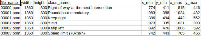
This should create the all_annots.csv file in the input directory with the following content structure.
Figure 3. A few rows from the traffic sign dataset CSV file.
As you can see, it contains all the information for images and corresponding ground truth.
Executing split_train_valid.py
Now, we will execute the split_train_valid.py script that will create a train.csv and valid.csv file in the input directory by randomly splitting the all_annots.csv file.
"""
Script to create a training and validation CSV file.
"""

import pandas as pd
import shutil
import os

def train_valid_split(all_images_folder=None, all_annots_csv=None, split=0.15):
    all_df = pd.read_csv(all_annots_csv)
    # Shuffle the CSV file rows.
    all_df.sample(frac=1)
    len_df = len(all_df)
    train_split = int((1-split)*len_df)

    train_df = all_df[:train_split]
    valid_df = all_df[train_split:]

    os.makedirs('../input/train_images', exist_ok=True)
    os.makedirs('../input/valid_images', exist_ok=True)

    # Copy training images.
    train_images = train_df['file_name'].tolist()
    for image in train_images:
        shutil.copy(
            f"../input/TrainIJCNN2013/{image}",
            f"../input/train_images/{image}"
        )
    train_df.to_csv('../input/train.csv', index=False)

    # Copy validation images.
    valid_images = valid_df['file_name'].tolist()
    for image in valid_images:
        shutil.copy(
            f"../input/TrainIJCNN2013/{image}",
            f"../input/valid_images/{image}"
        )
    valid_df.to_csv('../input/valid.csv', index=False)

train_valid_split(all_annots_csv='../input/all_annots.csv')
Execute the script from the src directory.
python split_train_valid.py
Executing csv_to_xml.py Script
This is the final data processing script. This will create the XML files for training and validation which will contain all the information and annotations for a particular image.
The content of csv_to_xml.py has been inspired from this code repository and modified according to our use case:
You can execute the script using the following command.
python csv_to_xml.py
This will create two directories, train_xmls and valid_xmls containing the training and validation XML files. The following block shows the content of one such XML file.
According to the current dataset splitting, we are using 15% of the data for validation and the rest for training. This amounts to 425 training examples and 81 validation examples.
Python Files in torch_utils Directory
mAP (Mean Average Precision) is one of the most common metrics to evaluate object detection models. But implementing the code for mAP from scratch can be tricky at times. Here, we will not be reinventing the wheel and implementing them from scratch. Instead, we will take help from the very reliable PyTorch detection repository and make a few changes according to our task. The same goes for the training and evaluation functions.
The torch_utils directory holds four Python files. Let’s go over them in brief.
coco_val.py: This contains the code for AP (Average Precision) and AR (Average Recall) calculation according to the MS COCO dataset standard.
coco_utils.py: This Python file contains the helper functions and classes that are used in the validation loop of engine.py to initialize the COCO API.
utils.py: We also need classes and functions for logging of the metrics and calculation of losses. The utils.py contains the code for that.
engine.py: This is like the training driver Python file. It contains the functions for training and validation loops. Those are train_one_epoch() and evaluate() functions.
Be sure to take a look at the above file before moving ahead. This will provide much more clarity on the internal working of the object detection code.
Model Files in the models Directory
You may notice that the models directory contains three Python files. Each of these three contains the create_model() function that will load the respective PyTorch Faster RCNN model for traffic sign detection.
fasterrcnn_resnet50.py: This will load fasterrcnn_resnet50_fpn() model upon calling the function. Out of three model code here, this is perhaps the best model in terms of mAP, yet the slowest in terms of FPS. This is because the ResNet50 backbone is quite large for it to be real-time.
fasterrcnn_mobilenetv3_large_fpn.py: This loads the Faster RCNN model with the MobileNetV3 Large FPN backbone model. In terms of speed, this is much faster than the ResNet50 Faster RCNN model but inferior in terms of performance (mAP).
fasterrcnn_mobilenetv3_large_320_fpn.py: This model is quite similar to the above one but internally resizes the images to a lower resolution, that is 320 pixels. It is the fastest of the three but also does not perform very well on smaller objects and when not having enough data for training.
For this post, primarily we will train the fasterrcnn_mobilenet_v3_large_fpn model. This should give us a good balance between accuracy and speed and will also allow us to perform inference on videos with good enough FPS. But as the code contains two other models, you can just switch the models any time you want and experiment quite easily on your own. Just as a heads up, the MobileNet 320 FPN one will not perform very well with this amount of data and also because the traffic signs are too small. But feel free to experiment with different augmentation techniques and try to improve the accuracy.
The datasets.py File to Prepare PyTorch Datasets and Data Loaders
In the src directory, the datasets.py contains the custom dataset class and functions to load the training and validation data loaders. In its current state, you can load any object detection dataset that you want. You just need to make sure that you have the images and XML files we had prepared earlier. Also, the custom dataset class supports loading different image formats like JPG, JPEG, PNG, and PPM.
We will not go into the details of the custom dataset class here. But it is very similar to the one described in this post. So, if you are interested in getting an in-depth explanation, please visit the link.
The custom_utils.py File
In short, the custom_utils.py contains a lot of helper functions and classes. These range from:
Helper functions to save the model.
To save images.
Annotate images with bounding boxes and text.
And even load the training and validation transforms and augmentation.
Out of all these, we will go through the training transforms and augmentations in detail here. The following code block contains the get_train_transform() function which transforms and augments the training data.
We are applying four different augmentations here. They are:
MotionBlur: To replicate the effect of an image taken from a speeding vehicle.
Blur: Randonly blurring the images.
RandomBrightnessContrast: To introduce different brightness and contrast intensities.
ColorJitter: To change the color of the images.
The above augmentations should introduce enough variability into the training dataset to train a robust model. If you intend to change the augmentations or add new ones, you need to be a bit careful. Some of the traffic signs are already pretty small and adding unnecessary augmentations can make the dataset a bit too difficult to learn. For example, we are not adding any flipping here. This is because flipping of traffic signs can render the entire object meaningless. Especially, flipping of the speed signs should be completely avoided.
After adding the augmentations, we are converting the images to tensors, and also adding the same set of augmentations to the bounding boxes (if applicable) using the bbox_params argument.
The Configuration (config.py) File
Next is the config.py file. This will define all the training configurations that we need. Let’s take a look at the content of the file first.
import torch

BATCH_SIZE = 4 # increase / decrease according to GPU memeory
RESIZE_TO = 512 # resize the image for training and transforms
NUM_EPOCHS = 200 # number of epochs to train for
NUM_WORKERS = 4

DEVICE = torch.device('cuda') if torch.cuda.is_available() else torch.device('cpu')

# Images and labels direcotry should be relative to train.py
TRAIN_DIR_IMAGES = '../input/train_images'
TRAIN_DIR_LABELS = '../input/train_xmls'
VALID_DIR_IMAGES = '../input/valid_images'
VALID_DIR_LABELS = '../input/valid_xmls'

# classes: 0 index is reserved for background
CLASSES = [
    '__background__',
    'Speed limit (20km/h)', 'Speed limit (30km/h)', 'Speed limit (50km/h)',
    'Speed limit (60km/h)', 'Speed limit (70km/h)', 'Speed limit (80km/h)',
    'End of speed limit (80km/h)', 'Speed limit (100km/h)',
    'Speed limit (120km/h)', 'No passing',
    'No passing for vehicles over 3.5 metric tons',
    'Right-of-way at the next intersection', 'Priority road', 'Yield',
    'Stop', 'No vehicles', 'Vehicles over 3.5 metric tons prohibited',
    'No entry', 'General caution', 'Dangerous curve to the left',
    'Dangerous curve to the right', 'Double curve', 'Bumpy road',
    'Slippery road', 'Road narrows on the right', 'Road work',
    'Traffic signals', 'Pedestrians', 'Children crossing',
    'Bicycles crossing', 'Beware of ice/snow', 'Wild animals crossing',
    'End of all speed and passing limits', 'Turn right ahead',
    'Turn left ahead', 'Ahead only', 'Go straight or right',
    'Go straight or left', 'Keep right', 'Keep left', 'Roundabout mandatory',
    'End of no passing', 'End of no passing by vehicles over 3.5 metric tons'
]

NUM_CLASSES = len(CLASSES)

# whether to visualize images after creating the data loaders
VISUALIZE_TRANSFORMED_IMAGES = False

# location to save model and plots
OUT_DIR = '../outputs'
As we can see, we define almost all the training configurations here. We have the batch size, the image size for resizing during dataset processing, the number of epochs to train for, and the number of workers as well.
Then we have the paths for training and validation images and also the XML files. We have the CLASSES list defining all the class names. Note that for Faster RCNN model training, the first class has to be the __background__ class that is present in our list as well.
There is another VISUALIZE_TRANSFORMED_IMAGES constant. If this is True, the program will show a few transformed images before the training begins. This is just to check what kind of images the model sees during training. The code for this is in the custom_utils.py file.
Finally, the OUT_DIR defines where the loss plots and trained models will be saved.
The train.py Script
There is just one other Python file we need to deal with before we can begin the traffic sign detection training using PyTorch and Faster RCNN.
It is the train.py script. This is the executable driver script.
The next code block contains the import statements for train.py.
from torch_utils.engine import (
    train_one_epoch, evaluate
)
from config import (
    DEVICE, NUM_CLASSES,
    NUM_EPOCHS, NUM_WORKERS,
    OUT_DIR, VISUALIZE_TRANSFORMED_IMAGES
)
from datasets import (
    create_train_dataset, create_valid_dataset,
    create_train_loader, create_valid_loader
)
from models.fasterrcnn_mobilenetv3_large_fpn import create_model
from custom_utils import (
    save_model,
    save_train_loss_plot,
    Averager, show_tranformed_image
)

import torch
As discussed earlier, we will train the MobileNetV3 Large FPN Faster RCNN model.
Now, we have the rest of the code under the main block.
if __name__ == '__main__':
    train_dataset = create_train_dataset()
    valid_dataset = create_valid_dataset()
    train_loader = create_train_loader(train_dataset, NUM_WORKERS)
    valid_loader = create_valid_loader(valid_dataset, NUM_WORKERS)
    print(f"Number of training samples: {len(train_dataset)}")
    print(f"Number of validation samples: {len(valid_dataset)}\n")

    if VISUALIZE_TRANSFORMED_IMAGES:
        show_tranformed_image(train_loader)

    # Initialize the Averager class.
    train_loss_hist = Averager()
    # Train and validation loss lists to store loss values of all
    # iterations till ena and plot graphs for all iterations.
    train_loss_list = []

    # Initialize the model and move to the computation device.
    model = create_model(num_classes=NUM_CLASSES)
    model = model.to(DEVICE)
    # Total parameters and trainable parameters.
    total_params = sum(p.numel() for p in model.parameters())
    print(f"{total_params:,} total parameters.")
    total_trainable_params = sum(
        p.numel() for p in model.parameters() if p.requires_grad)
    print(f"{total_trainable_params:,} training parameters.\n")
    # Get the model parameters.
    params = [p for p in model.parameters() if p.requires_grad]
    # Define the optimizer.
    # optimizer = torch.optim.SGD(params, lr=0.001, momentum=0.9, weight_decay=0.0005)
    optimizer = torch.optim.AdamW(params, lr=0.0001, weight_decay=0.0005)

    # LR will be zero as we approach `steps` number of epochs each time.
    # If `steps = 5`, LR will slowly reduce to zero every 5 epochs.
    steps = NUM_EPOCHS + 25
    scheduler = torch.optim.lr_scheduler.CosineAnnealingWarmRestarts(
        optimizer,
        T_0=steps,
        T_mult=1,
        verbose=True
    )

    for epoch in range(NUM_EPOCHS):
        train_loss_hist.reset()

        _, batch_loss_list = train_one_epoch(
            model,
            optimizer,
            train_loader,
            DEVICE,
            epoch,
            train_loss_hist,
            print_freq=100,
            scheduler=scheduler
        )

        evaluate(model, valid_loader, device=DEVICE)

        # Add the current epoch's batch-wise lossed to the `train_loss_list`.
        train_loss_list.extend(batch_loss_list)

        # Save the current epoch model.
        save_model(OUT_DIR, epoch, model, optimizer)

        # Save loss plot.
        save_train_loss_plot(OUT_DIR, train_loss_list)
Let’s focus on the important stuff here.
First is the optimizer. We are using the AdamW optimizer instead of SGD here. From the experiments, I found that the AdamW optimizer combined with CosineAnnealingWarmRestarts gave slightly lower loss and seems to improve the inference predictions also.
On similar line, we are using the CosineAnnealingWarmRestarts for learning rate scheduling here. You may notice that we are training for 200 epochs, but the first learning rate restart will happen at epoch number 225. This is just to ensure that the learning rate keeps on reducing by the same amount with each iteration and stays slightly above 0 the last few epochs. This strategy seems to improve the mAP a bit.
After that we have the for loop starting the training and evaluation for 200 epochs.
After every epoch we save the current model and the training loss plot to disk.
Although we did not go into much of the coding details here, still, it was a lot to cover in terms of the entire training pipeline. Now, we are all set to start the training for traffic sign detection using PyTorch and Faster RCNN.
Executing train.py for Traffic Sign Detection using PyTorch and Faster RCNN
Open your terminal/command line in the src directory and execute the train.py script. If you are training locally, make sure that you have a GPU. Even if you cannot train the model, you have access to the trained model when you download the zip file for the post. So, you can run the inference without any issues.
python train.py
The following is the truncated output from the terminal.
Number of training samples: 425
Number of validation samples: 81

19,145,479 total parameters.
19,086,583 training parameters.

Epoch     0: adjusting learning rate of group 0 to 1.0000e-04.
Epoch: [0]  [  0/107]  eta: 0:01:26  lr: 0.000001  loss: 4.0942 (4.0942)  loss_classifier: 3.9772 (3.9772)  loss_box_reg: 0.0659 (0.0659)  loss_objectness: 0.0467 (0.0467)  loss_rpn_box_reg: 0.0044 (0.0044)  time: 0.8070  data: 0.2524  max mem: 966
Epoch: [0]  [100/107]  eta: 0:00:00  lr: 0.000101  loss: 0.4165 (0.5722)  loss_classifier: 0.2571 (0.4177)  loss_box_reg: 0.1338 (0.1322)  loss_objectness: 0.0123 (0.0175)  loss_rpn_box_reg: 0.0044 (0.0048)  time: 0.0637  data: 0.0056  max mem: 1183
Epoch: [0]  [106/107]  eta: 0:00:00  lr: 0.000100  loss: 0.4658 (0.5756)  loss_classifier: 0.3119 (0.4180)  loss_box_reg: 0.1559 (0.1359)  loss_objectness: 0.0110 (0.0169)  loss_rpn_box_reg: 0.0043 (0.0049)  time: 0.0598  data: 0.0051  max mem: 1183
Epoch: [0] Total time: 0:00:07 (0.0706 s / it)
creating index...
index created!
Test:  [ 0/21]  eta: 0:00:03  model_time: 0.0253 (0.0253)  evaluator_time: 0.0019 (0.0019)  time: 0.1899  data: 0.1577  max mem: 1183
Test:  [20/21]  eta: 0:00:00  model_time: 0.0234 (0.0230)  evaluator_time: 0.0019 (0.0019)  time: 0.0305  data: 0.0041  max mem: 1183
Test: Total time: 0:00:00 (0.0398 s / it)
Averaged stats: model_time: 0.0234 (0.0230)  evaluator_time: 0.0019 (0.0019)
Accumulating evaluation results...
DONE (t=0.05s).
IoU metric: bbox
 Average Precision  (AP) @[ IoU=0.50:0.95 | area=   all | maxDets=100 ] = 0.022
 Average Precision  (AP) @[ IoU=0.50      | area=   all | maxDets=100 ] = 0.041
 Average Precision  (AP) @[ IoU=0.75      | area=   all | maxDets=100 ] = 0.030
 Average Precision  (AP) @[ IoU=0.50:0.95 | area= small | maxDets=100 ] = 0.015
 Average Precision  (AP) @[ IoU=0.50:0.95 | area=medium | maxDets=100 ] = 0.178
 Average Precision  (AP) @[ IoU=0.50:0.95 | area= large | maxDets=100 ] = -1.000
 Average Recall     (AR) @[ IoU=0.50:0.95 | area=   all | maxDets=  1 ] = 0.051
 Average Recall     (AR) @[ IoU=0.50:0.95 | area=   all | maxDets= 10 ] = 0.052
 Average Recall     (AR) @[ IoU=0.50:0.95 | area=   all | maxDets=100 ] = 0.052
 Average Recall     (AR) @[ IoU=0.50:0.95 | area= small | maxDets=100 ] = 0.042
 Average Recall     (AR) @[ IoU=0.50:0.95 | area=medium | maxDets=100 ] = 0.178
 Average Recall     (AR) @[ IoU=0.50:0.95 | area= large | maxDets=100 ] = -1.000
SAVING PLOTS COMPLETE...
...
Epoch: [199]  [  0/107]  eta: 0:00:31  lr: 0.000004  loss: 0.2822 (0.2822)  loss_classifier: 0.1035 (0.1035)  loss_box_reg: 0.1786 (0.1786)  loss_objectness: 0.0001 (0.0001)  loss_rpn_box_reg: 0.0000 (0.0000)  time: 0.2901  data: 0.2335  max mem: 1183
Epoch: [199]  [100/107]  eta: 0:00:00  lr: 0.000003  loss: 0.2186 (0.2498)  loss_classifier: 0.0370 (0.0491)  loss_box_reg: 0.2090 (0.2003)  loss_objectness: 0.0001 (0.0002)  loss_rpn_box_reg: 0.0000 (0.0001)  time: 0.0546  data: 0.0052  max mem: 1183
Epoch: [199]  [106/107]  eta: 0:00:00  lr: 0.000003  loss: 0.2169 (0.2474)  loss_classifier: 0.0388 (0.0486)  loss_box_reg: 0.1840 (0.1984)  loss_objectness: 0.0001 (0.0002)  loss_rpn_box_reg: 0.0001 (0.0001)  time: 0.0528  data: 0.0050  max mem: 1183
Epoch: [199] Total time: 0:00:06 (0.0571 s / it)
creating index...
index created!
Test:  [ 0/21]  eta: 0:00:04  model_time: 0.0243 (0.0243)  evaluator_time: 0.0023 (0.0023)  time: 0.2298  data: 0.2007  max mem: 1183
Test:  [20/21]  eta: 0:00:00  model_time: 0.0221 (0.0217)  evaluator_time: 0.0026 (0.0024)  time: 0.0308  data: 0.0050  max mem: 1183
Test: Total time: 0:00:00 (0.0431 s / it)
Averaged stats: model_time: 0.0221 (0.0217)  evaluator_time: 0.0026 (0.0024)
Accumulating evaluation results...
DONE (t=0.06s).
IoU metric: bbox
 Average Precision  (AP) @[ IoU=0.50:0.95 | area=   all | maxDets=100 ] = 0.210
 Average Precision  (AP) @[ IoU=0.50      | area=   all | maxDets=100 ] = 0.323
 Average Precision  (AP) @[ IoU=0.75      | area=   all | maxDets=100 ] = 0.212
 Average Precision  (AP) @[ IoU=0.50:0.95 | area= small | maxDets=100 ] = 0.227
 Average Precision  (AP) @[ IoU=0.50:0.95 | area=medium | maxDets=100 ] = 0.534
 Average Precision  (AP) @[ IoU=0.50:0.95 | area= large | maxDets=100 ] = -1.000
 Average Recall     (AR) @[ IoU=0.50:0.95 | area=   all | maxDets=  1 ] = 0.293
 Average Recall     (AR) @[ IoU=0.50:0.95 | area=   all | maxDets= 10 ] = 0.300
 Average Recall     (AR) @[ IoU=0.50:0.95 | area=   all | maxDets=100 ] = 0.300
 Average Recall     (AR) @[ IoU=0.50:0.95 | area= small | maxDets=100 ] = 0.283
 Average Recall     (AR) @[ IoU=0.50:0.95 | area=medium | maxDets=100 ] = 0.583
 Average Recall     (AR) @[ IoU=0.50:0.95 | area= large | maxDets=100 ] = -1.000
SAVING PLOTS COMPLETE...
After 200 epochs, the mAP for 0.5 IoU is 32.3% and for for IoU=0.50:0.95 is 21.0%. This is not very great but not too terrible either. If you remember, the objects are small and quite difficult as well. And the model backbone is MobileNetV3.
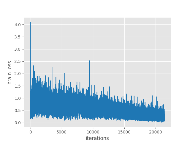
The following is the iteration-wise loss graph that is saved to disk.
Figure 4. Loss after training the PyTorch Faster RCNN model.
The training loss was decreasing till the end of training. Perhaps a few more epochs of training would have helped as well. But let’s use this model for now to run the inference.
Inference using the Trained Faster RCNN Model
First, we will run inference on images, then inference on videos. We have two different scripts for this. One is inference.py for running inference on images and inference_video.py for running inference on videos.
Both the image inference and video inference were run on a machine with RTX 3080 GPU (10 GB), 32 GB RAM, and a 10th generation i7 processor.
Running Inference on Images for Traffic Sign Detection using PyTorch
Before running the script, be sure to take a few minutes and go through the inference.py script. A few important features of the script:
It can either take path to a directory containing images or even a single image file. We can provide either of two from the command line using the --input flag.
We can also provide an integer using the --resize flag. Use this either to resize the image to a larger or smaller size. For example, providing 300 will resize it to 300×300.
Also, it supports multiple image formats for a directory path which include, JPG, JPEG, PNG, and PPM.
We will be carrying out inference on the test images present in the input/TestIJCNN2013/TestIJCNN2013Download directory.
Execute the following command within the src directory.
The average FPS on all the images was around 73 which is pretty good considering it is a Faster RCNN model. This is most likely due to the lighter MobileNetV3 Large backbone.
We can see that the model predicts traffic signs like Keep right, Speed limit (50km/h), and Speed limit (30km/h) correctly most of the time.
However, it is making mistakes if the traffic sign is too small or if they are similar like Slippery road, Beware of ice/snow.
It might be just that the MobileNetV3 Large backbone is not good enough for this task. The small number of training examples can also be an issue. Still, let’s move ahead with the video inference.
Running Inference on Videos
While executing the inference_video.py, we need to provide the path to the input video file. Also, it supports the same resizing format as the image inference script.
Execute the following for running inference on video.
Clip 1. Traffic sign detection video inference using MobileNetV3 Large FPN Faster RCNN model.
The inference on video is good only when the traffic sign is too close. Shadows and smaller traffic signs are resulting in wrong predictions. Also, when the traffic signs are far away, we can see a lot of fluctuations. This clearly shows the limitation of using a smaller backbone like MobileNetV3.
Results using ResNet50 FPN Faster RCNN Model
Just for the sake of comparison, the following are the results using fasterrcnn_resnet50_fpn model.
python train.py
Number of training samples: 425
Number of validation samples: 81

41,514,411 total parameters.
41,292,011 training parameters.

Epoch     0: adjusting learning rate of group 0 to 1.0000e-04.
/home/sovit/miniconda3/envs/torch110/lib/python3.9/site-packages/torch/functional.py:445: UserWarning: torch.meshgrid: in an upcoming release, it will be required to pass the indexing argument. (Triggered internally at  /opt/conda/conda-bld/pytorch_1634272204863/work/aten/src/ATen/native/TensorShape.cpp:2157.)
  return _VF.meshgrid(tensors, **kwargs)  # type: ignore[attr-defined]
Epoch: [0]  [  0/107]  eta: 0:03:04  lr: 0.000001  loss: 4.1653 (4.1653)  loss_classifier: 4.0820 (4.0820)  loss_box_reg: 0.0356 (0.0356)  loss_objectness: 0.0462 (0.0462)  loss_rpn_box_reg: 0.0014 (0.0014)  time: 1.7221  data: 0.2689  max mem: 3007
Epoch: [0]  [100/107]  eta: 0:00:01  lr: 0.000101  loss: 0.3237 (0.5056)  loss_classifier: 0.1659 (0.3279)  loss_box_reg: 0.1106 (0.1345)  loss_objectness: 0.0145 (0.0326)  loss_rpn_box_reg: 0.0046 (0.0106)  time: 0.2310  data: 0.0051  max mem: 3433
Epoch: [0]  [106/107]  eta: 0:00:00  lr: 0.000100  loss: 0.3030 (0.4956)  loss_classifier: 0.1771 (0.3202)  loss_box_reg: 0.0941 (0.1332)  loss_objectness: 0.0167 (0.0318)  loss_rpn_box_reg: 0.0046 (0.0104)  time: 0.2231  data: 0.0049  max mem: 3433
Epoch: [0] Total time: 0:00:26 (0.2437 s / it)
creating index...
index created!
Test:  [ 0/21]  eta: 0:00:05  model_time: 0.1001 (0.1001)  evaluator_time: 0.0048 (0.0048)  time: 0.2562  data: 0.1471  max mem: 3433
Test:  [20/21]  eta: 0:00:00  model_time: 0.0980 (0.0949)  evaluator_time: 0.0041 (0.0042)  time: 0.1050  data: 0.0047  max mem: 3433
Test: Total time: 0:00:02 (0.1139 s / it)
Averaged stats: model_time: 0.0980 (0.0949)  evaluator_time: 0.0041 (0.0042)
Accumulating evaluation results...
DONE (t=0.07s).
IoU metric: bbox
 Average Precision  (AP) @[ IoU=0.50:0.95 | area=   all | maxDets=100 ] = 0.027
 Average Precision  (AP) @[ IoU=0.50      | area=   all | maxDets=100 ] = 0.060
 Average Precision  (AP) @[ IoU=0.75      | area=   all | maxDets=100 ] = 0.013
 Average Precision  (AP) @[ IoU=0.50:0.95 | area= small | maxDets=100 ] = 0.027
 Average Precision  (AP) @[ IoU=0.50:0.95 | area=medium | maxDets=100 ] = 0.113
 Average Precision  (AP) @[ IoU=0.50:0.95 | area= large | maxDets=100 ] = -1.000
 Average Recall     (AR) @[ IoU=0.50:0.95 | area=   all | maxDets=  1 ] = 0.089
 Average Recall     (AR) @[ IoU=0.50:0.95 | area=   all | maxDets= 10 ] = 0.122
 Average Recall     (AR) @[ IoU=0.50:0.95 | area=   all | maxDets=100 ] = 0.122
 Average Recall     (AR) @[ IoU=0.50:0.95 | area= small | maxDets=100 ] = 0.119
 Average Recall     (AR) @[ IoU=0.50:0.95 | area=medium | maxDets=100 ] = 0.272
 Average Recall     (AR) @[ IoU=0.50:0.95 | area= large | maxDets=100 ] = -1.000
SAVING PLOTS COMPLETE...
...
Epoch: [199]  [  0/107]  eta: 0:00:46  lr: 0.000004  loss: 0.0027 (0.0027)  loss_classifier: 0.0019 (0.0019)  loss_box_reg: 0.0008 (0.0008)  loss_objectness: 0.0000 (0.0000)  loss_rpn_box_reg: 0.0000 (0.0000)  time: 0.4340  data: 0.2040  max mem: 3433
Epoch: [199]  [100/107]  eta: 0:00:01  lr: 0.000003  loss: 0.0074 (0.0080)  loss_classifier: 0.0027 (0.0033)  loss_box_reg: 0.0034 (0.0044)  loss_objectness: 0.0000 (0.0001)  loss_rpn_box_reg: 0.0001 (0.0002)  time: 0.2263  data: 0.0051  max mem: 3433
Epoch: [199]  [106/107]  eta: 0:00:00  lr: 0.000003  loss: 0.0058 (0.0080)  loss_classifier: 0.0025 (0.0033)  loss_box_reg: 0.0029 (0.0044)  loss_objectness: 0.0000 (0.0001)  loss_rpn_box_reg: 0.0001 (0.0002)  time: 0.2185  data: 0.0050  max mem: 3433
Epoch: [199] Total time: 0:00:24 (0.2274 s / it)
creating index...
index created!
Test:  [ 0/21]  eta: 0:00:06  model_time: 0.0972 (0.0972)  evaluator_time: 0.0027 (0.0027)  time: 0.3000  data: 0.1973  max mem: 3433
Test:  [20/21]  eta: 0:00:00  model_time: 0.0961 (0.0930)  evaluator_time: 0.0023 (0.0023)  time: 0.1009  data: 0.0041  max mem: 3433
Test: Total time: 0:00:02 (0.1130 s / it)
Averaged stats: model_time: 0.0961 (0.0930)  evaluator_time: 0.0023 (0.0023)
Accumulating evaluation results...
DONE (t=0.07s).
IoU metric: bbox
 Average Precision  (AP) @[ IoU=0.50:0.95 | area=   all | maxDets=100 ] = 0.522
 Average Precision  (AP) @[ IoU=0.50      | area=   all | maxDets=100 ] = 0.636
 Average Precision  (AP) @[ IoU=0.75      | area=   all | maxDets=100 ] = 0.624
 Average Precision  (AP) @[ IoU=0.50:0.95 | area= small | maxDets=100 ] = 0.523
 Average Precision  (AP) @[ IoU=0.50:0.95 | area=medium | maxDets=100 ] = 0.611
 Average Precision  (AP) @[ IoU=0.50:0.95 | area= large | maxDets=100 ] = -1.000
 Average Recall     (AR) @[ IoU=0.50:0.95 | area=   all | maxDets=  1 ] = 0.613
 Average Recall     (AR) @[ IoU=0.50:0.95 | area=   all | maxDets= 10 ] = 0.663
 Average Recall     (AR) @[ IoU=0.50:0.95 | area=   all | maxDets=100 ] = 0.663
 Average Recall     (AR) @[ IoU=0.50:0.95 | area= small | maxDets=100 ] = 0.663
 Average Recall     (AR) @[ IoU=0.50:0.95 | area=medium | maxDets=100 ] = 0.661
 Average Recall     (AR) @[ IoU=0.50:0.95 | area= large | maxDets=100 ] = -1.000
SAVING PLOTS COMPLETE...
The loss is lower in this case and the mAP is also higher. This is expected as ResNet50 is a much larger backbone.
Further Steps
Further on, you can try running inference after training the ResNet50 FPN Faster RCNN model. You will surely get better results and be sure to share them in the comment section.
You can also try training the fasterrcnn_mobilenet_v3_large_320_fpn model and checking how it is performing.
Summary and Conclusion
We covered a lot of things for traffic sign detection using PyTorch and Faster RCNN in this post. We started with the exploration of the Python code files and then trained a Faster RCNN model with MobileNetV3 Large FPN backbone. During the inference, we got to know why the model is not able to perform very well and also that the ResNet50 Faster RCNN gives better mAP. In future posts, we will explore more such detections projects along this line. I hope that you learned something new from this post.
If you have any doubts, thoughts, or suggestions, please leave them in the comment section. I will surely address them.
You can contact me using the Contact section. You can also find me on LinkedIn, and X.
Credits for Video Used for Inference
Trimmed version of video_1.mp4 in input/inference_data: https://www.youtube.com/watch?v=vnqkraiSiTI
Liked it? Take a second to support Sovit Ranjan Rath on Patreon!
Really great explanation of the project. Can you give an idea on how can I calculate model accuracy metric from this and also any guide on building confusion matrix for the same?
Hello Akshit. In object detection, the mAP (Mean Average Precision) acts as the model accuracy. This is already shown in the blog post in the training section.
For the accuracy matrix, I will try to update the post.
In case you want more advanced and easier pipeline to train multiple Faster RCNN models, this GitHub repository is the best place in my opinion. https://github.com/sovit-123/fasterrcnn-pytorch-training-pipeline
Hello Noor Chauhan. Can you please try disabling ad blocker or DuckDuckGo if you have them enabled? It creates issues with the download code button. If that still does not work, please let me.
Hello, Thank you very much for the great tutorial. I have been trying to implement this, as well as this one (https://debuggercafe.com/custom-object-detection-using-pytorch-faster-rcnn/). I wanted to ask if it is possible to use other models for Faster R-CNN, such as DenseNet121 or ShuffleNet? And if so, any help would be appreciated.
Hello Viktoria. Yes, we can use almost any backbone from Torchvision with Faster RCNN head. I have creating a Faster RCNN Training Pipeline library which supports several backbones at the moment. Please check the library here => https://github.com/sovit-123/fasterrcnn-pytorch-training-pipeline
Thank you it worked.
Now I have the problem that the fps are very low like 0.1, 0.2 how can I raise it up?
I run the code on an Raspberry Pi 4 model b with 4gb of Ram.
I appreciate your help
Hello Ilkan. I am working on making Faster RCNN models even faster. I will be sharing the updates in my Faster RCNN training repository that you can find here. If you are planning on a long term project, please consider using this repository. It supports a host of features. https://github.com/sovit-123/fasterrcnn-pytorch-training-pipeline
Hello,I am a gree-hand.I have a question.I run 600 epochs,but when I test a video,the accuray is still very low.What should I do to improve it?Can you give me some advice?Thank you so much.
Can you let me know whether these results are from the MobileNet backbone one or are you using some other backbone? Mostly, if it is from the MobileNet backbone model, then I guess the results match up with the blog post more or less. Whatever mAP different is there, will be because of overfitting as you are training for 600 epochs.
The higher mAP numbers that I show at the end are from the Faster RCNN ResNet50 model. So, you may be confusing that and thinking that your mAP is low.
Hello. Apologies for the trouble. I have sent you an email with the download link.
Sometimes, ad blockers or DuckDuckGo may cause issues with the downloading process. Please try to disable them when trying to download and you can enable them again once the download completes.
I hope this helps.
Hello. I think I am a bit lost here. If you are asking about the model, then the entire architecture is available in the model.py after downloading the content for this article.
I hope this helps.
When I try to use image inference on the model, I end up getting this error. Are there any ways to fix this? I saw some other people have the same issue online but their fixes did not work for me. Thanks!
/usr/local/lib/python3.10/dist-packages/torchvision/models/_utils.py:208: UserWarning: The parameter ‘pretrained’ is deprecated since 0.13 and may be removed in the future, please use ‘weights’ instead.
warnings.warn(
/usr/local/lib/python3.10/dist-packages/torchvision/models/_utils.py:223: UserWarning: Arguments other than a weight enum or `None` for ‘weights’ are deprecated since 0.13 and may be removed in the future. The current behavior is equivalent to passing `weights=FasterRCNN_MobileNet_V3_Large_FPN_Weights.COCO_V1`. You can also use `weights=FasterRCNN_MobileNet_V3_Large_FPN_Weights.DEFAULT` to get the most up-to-date weights.
warnings.warn(msg)
Traceback (most recent call last):
File “/content/r50/20220404_Traffic_Sign_Detection_using_PyTorch_and_Pretrained_Faster_RCNN_Model/src/inference.py”, line 41, in
model.load_state_dict(checkpoint[‘model_state_dict’])
File “/usr/local/lib/python3.10/dist-packages/torch/nn/modules/module.py”, line 2041, in load_state_dict
raise RuntimeError(‘Error(s) in loading state_dict for {}:\n\t{}’.format(
RuntimeError: Error(s) in loading state_dict for FasterRCNN:
Missing key(s) in state_dict: “backbone.body.0.0.weight”, “backbone.body.0.1.weight”, “backbone.body.0.1.bias”, “backbone.body.0.1.running_mean”… (truncated)
Are you running the training and inference on the same dataset as the post or a different one? It seems that the mode which has been saved and the model which loads up for inference are different. That’s why the weight layers do not match.
I am running it on the same dataset yes. I also tried training R50, and then using the R50 model that was output after training, and got that error as well.
Hi. I checked the code and it is running fine. From your file path, it seems like you are loading the Faster RCNN ResNet50 weights while initializing the Faster RCNN MobileNetV3 Large Model. Please take a look if that is the case. The training and inference files initialize the Faster RCNN MobileNetV3 large model and not the ResNet50 one. So, the Faster RCNN MobileNetV3 Large weights should be loaded. Please check that the model that you are initializing and the weights that you are loading match.
I am running the code on Google Collab, but it shows error “ImportError: cannot import name ‘DEVICE’ from ‘config’ (/usr/local/lib/python3.10/dist-packages/config/__init__.py)”. Then, I tried to import the necessary libraries and proceeded with the following codes. However, now it shows “TypeError: train_one_epoch() got multiple values for argument ‘print_freq'”
ok, thanks! I managed to run the code in my local machine. However, may I ask if I am on the right track? After I run the train.py, it kept adjusting the learning rate tho.
Epoch 00000: adjusting learning rate of group 0 to 1.0000e-04.
Epoch 0.00: adjusting learning rate of group 0 to 1.0000e-04.
Epoch: [0] [ 0/107] eta: 2:22:17 lr: 0.000001 loss: 4.1082 (4.1082) loss_classifier: 4.0117 (4.0117) loss_box_reg: 0.0441 (0.0441) loss_objectness: 0.0479 (0.0479) loss_rpn_box_reg: 0.0044 (0.0044) time: 79.7934 data: 21.1116
Epoch 0.00: adjusting learning rate of group 0 to 1.0000e-04.
Epoch 0.00: adjusting learning rate of group 0 to 1.0000e-04.
Epoch 0.00: adjusting learning rate of group 0 to 1.0000e-04.
hi i have a question, for the testing set, it only shows the plotting of the bounding boxes and a graph of train loss right? How can I determine the mAP values for the testing set?
Hi. The inference.py script is only meant for running inference and detection on new data. It will not be able to provide mAP as it does not have access to the ground truth data.
Hi, I understand that there’s no ground truth data for this particular tutorial. Do you have any suggestions or any other tutorials that has a script to run inference on a test set with ground truth data to calculate the mAP? thank you.
Thanks for sharing, but my run of the model encountered KeyError: tensor(9) (where the number is different each time), I checked the txt file already csv file, the content is correct, please tell me what’s wrong!
Hi Amin. Can you please try disabling adblocker or DuckDuckGo when downloading if you have them enabled? If you have DuckDuckGo, please remove this URL, it blocks all APIs for some reason. Let me know if this works.
This website uses cookies so that we can provide you with the best user experience possible. Cookie information is stored in your browser and performs functions such as recognising you when you return to our website and helping our team to understand which sections of the website you find most interesting and useful.
Strictly Necessary Cookies
Strictly Necessary Cookie should be enabled at all times so that we can save your preferences for cookie settings.
If you disable this cookie, we will not be able to save your preferences. This means that every time you visit this website you will need to enable or disable cookies again.


Can I get the research papers that were used for this project?
Hello Zachary.
I think the most important one is going through the Faster RCNN paper => https://arxiv.org/abs/1506.01497
Also, you can take a look at the dataset website => https://benchmark.ini.rub.de/
Really great explanation of the project. Can you give an idea on how can I calculate model accuracy metric from this and also any guide on building confusion matrix for the same?
Hello Akshit. In object detection, the mAP (Mean Average Precision) acts as the model accuracy. This is already shown in the blog post in the training section.
For the accuracy matrix, I will try to update the post.
In case you want more advanced and easier pipeline to train multiple Faster RCNN models, this GitHub repository is the best place in my opinion.
https://github.com/sovit-123/fasterrcnn-pytorch-training-pipeline
Hi the link to download the source code doesn’t seem to be working
Hello Lucas. I have sent a reply to you on your email. Please check.
Hi, the download source code button doesn’t work.
Hello. In have sent the link as in an email to you. Please check. I hope this solves your issue.
Hi, the download source code button isnt working, how do we proceed to download it?
Hello Noor Chauhan. Can you please try disabling ad blocker or DuckDuckGo if you have them enabled? It creates issues with the download code button. If that still does not work, please let me.
Hello, Thank you very much for the great tutorial. I have been trying to implement this, as well as this one (https://debuggercafe.com/custom-object-detection-using-pytorch-faster-rcnn/). I wanted to ask if it is possible to use other models for Faster R-CNN, such as DenseNet121 or ShuffleNet? And if so, any help would be appreciated.
Hello Viktoria. Yes, we can use almost any backbone from Torchvision with Faster RCNN head. I have creating a Faster RCNN Training Pipeline library which supports several backbones at the moment. Please check the library here =>
https://github.com/sovit-123/fasterrcnn-pytorch-training-pipeline
You will find all the supported Faster RCNN models at the end of the README file.
Or you can directly click here => https://github.com/sovit-123/fasterrcnn-pytorch-training-pipeline#A-List-of-All-Model-Flags-to-Use-With-the-Training-Script
Hello Sir,Could you please provide me the architecture of fasterrcnn_mobilenet_v3_large_fpn
Hello Muhammad. Can you please elaborate what you mean by proving the architecture?
In case you are looking to train using the model, then please take a look at this repository => https://github.com/sovit-123/fasterrcnn-pytorch-training-pipeline
It is extremely easy to train and contains the architecture that you are looking for. I think this will solve your issue.
Hello, is it possible to change the video input to a live camera input?
And if so, any help would be appreciated.
You can just change the code inference script to cv2.VideoCapture(0). Change it in the inference_video.py file.
Thank you it worked.
Now I have the problem that the fps are very low like 0.1, 0.2 how can I raise it up?
I run the code on an Raspberry Pi 4 model b with 4gb of Ram.
I appreciate your help
Hello Ilkan. I am working on making Faster RCNN models even faster. I will be sharing the updates in my Faster RCNN training repository that you can find here. If you are planning on a long term project, please consider using this repository. It supports a host of features.
https://github.com/sovit-123/fasterrcnn-pytorch-training-pipeline
I’m not sure about the custom_utils.py File. Can you help with the complete code of that file.
Hello David, all the content and files are present in the downloadable zip file. Please download it. You will get all the files.
Hello,I am a gree-hand.I have a question.I run 600 epochs,but when I test a video,the accuray is still very low.What should I do to improve it?Can you give me some advice?Thank you so much.
Hello. Can you let me know what the final mAP if and if you can also show me the mAP graphs somehow?
Thanks for your reply.I don’t know how to calculate mAP.I get the train result only.
Are you meaning these?
Epoch 599.00: adjusting learning rate of group 0 to 4.2639e-07.
Epoch: [599] [0/8] eta: 0:01:11 lr: 0.000000 loss: 0.1516 (0.1516) loss_classifier: 0.0161 (0.0161) loss_box_reg: 0.1353 (0.1353) loss_objectness: 0.0002 (0.0002) loss_rpn_box_reg: 0.0001 (0.0001) time: 8.9654 data: 6.7667 max mem: 11525
Epoch 599.00: adjusting learning rate of group 0 to 4.2639e-07.
Epoch 599.00: adjusting learning rate of group 0 to 4.2639e-07.
Epoch 599.00: adjusting learning rate of group 0 to 4.2639e-07.
Epoch 599.00: adjusting learning rate of group 0 to 4.2639e-07.
Epoch 599.00: adjusting learning rate of group 0 to 4.2639e-07.
Epoch 599.00: adjusting learning rate of group 0 to 4.2639e-07.
Epoch 599.00: adjusting learning rate of group 0 to 4.2639e-07.
Epoch: [599] [7/8] eta: 0:00:02 lr: 0.000000 loss: 0.1937 (0.1962) loss_classifier: 0.0459 (0.0439) loss_box_reg: 0.1487 (0.1520) loss_objectness: 0.0002 (0.0003) loss_rpn_box_reg: 0.0001 (0.0001) time: 2.5802 data: 1.0090 max mem: 11525
Epoch: [599] Total time: 0:00:20 (2.5963 s / it)
creating index…
index created!
Test: [0/2] eta: 0:00:05 model_time: 0.7419 (0.7419) evaluator_time: 0.0714 (0.0714) time: 2.6248 data: 1.7594 max mem: 11525
Test: [1/2] eta: 0:00:01 model_time: 0.3517 (0.5468) evaluator_time: 0.0334 (0.0524) time: 1.5390 data: 0.8976 max mem: 11525
Test: Total time: 0:00:03 (1.6318 s / it)
Averaged stats: model_time: 0.3517 (0.5468) evaluator_time: 0.0334 (0.0524)
Accumulating evaluation results…
DONE (t=0.16s).
IoU metric: bbox
Average Precision (AP) @[ IoU=0.50:0.95 | area= all | maxDets=100 ] = 0.156
Average Precision (AP) @[ IoU=0.50 | area= all | maxDets=100 ] = 0.261
Average Precision (AP) @[ IoU=0.75 | area= all | maxDets=100 ] = 0.143
Average Precision (AP) @[ IoU=0.50:0.95 | area= small | maxDets=100 ] = 0.157
Average Precision (AP) @[ IoU=0.50:0.95 | area=medium | maxDets=100 ] = 0.304
Average Precision (AP) @[ IoU=0.50:0.95 | area= large | maxDets=100 ] = -1.000
Average Recall (AR) @[ IoU=0.50:0.95 | area= all | maxDets= 1 ] = 0.198
Average Recall (AR) @[ IoU=0.50:0.95 | area= all | maxDets= 10 ] = 0.201
Average Recall (AR) @[ IoU=0.50:0.95 | area= all | maxDets=100 ] = 0.201
Average Recall (AR) @[ IoU=0.50:0.95 | area= small | maxDets=100 ] = 0.188
Average Recall (AR) @[ IoU=0.50:0.95 | area=medium | maxDets=100 ] = 0.317
Average Recall (AR) @[ IoU=0.50:0.95 | area= large | maxDets=100 ] = -1.000
SAVING PLOTS COMPLETE…
Can you let me know whether these results are from the MobileNet backbone one or are you using some other backbone? Mostly, if it is from the MobileNet backbone model, then I guess the results match up with the blog post more or less. Whatever mAP different is there, will be because of overfitting as you are training for 600 epochs.
The higher mAP numbers that I show at the end are from the Faster RCNN ResNet50 model. So, you may be confusing that and thinking that your mAP is low.
Hie the button to the source code is not working
Hello. I have sent you an email with the download link. Please check.
Hello is there a way to change the training transformations cuz I am getting an error when trying to change them
Hello Anon. What is the error that you are getting?
Hello thanks for this beautiful work, the button to the source code is not working 🙁
Hello. Apologies for the trouble. I have sent you an email with the download link.
Sometimes, ad blockers or DuckDuckGo may cause issues with the downloading process. Please try to disable them when trying to download and you can enable them again once the download completes.
I hope this helps.
thanks, this helps alot.
Welcome.
Can you give me the model classes? I want to put this project on FPGA.
such as max pooling, fully connected.
Hello. I think I am a bit lost here. If you are asking about the model, then the entire architecture is available in the model.py after downloading the content for this article.
I hope this helps.
hello can you please send me the source code?
Hello Ramin. I have sent the link to your email. Please check.
Hello, can you send me the source code?
Hello. I have sent an email. Please check and let me know.
Hi, how do I import the faster rcnn resnet50 model instead of the mobilenet one? I get a module not found error when i try.
nevermind i fixed it
Glad that you fixed it.
Hi,
When I try to use image inference on the model, I end up getting this error. Are there any ways to fix this? I saw some other people have the same issue online but their fixes did not work for me. Thanks!
/usr/local/lib/python3.10/dist-packages/torchvision/models/_utils.py:208: UserWarning: The parameter ‘pretrained’ is deprecated since 0.13 and may be removed in the future, please use ‘weights’ instead.
warnings.warn(
/usr/local/lib/python3.10/dist-packages/torchvision/models/_utils.py:223: UserWarning: Arguments other than a weight enum or `None` for ‘weights’ are deprecated since 0.13 and may be removed in the future. The current behavior is equivalent to passing `weights=FasterRCNN_MobileNet_V3_Large_FPN_Weights.COCO_V1`. You can also use `weights=FasterRCNN_MobileNet_V3_Large_FPN_Weights.DEFAULT` to get the most up-to-date weights.
warnings.warn(msg)
Traceback (most recent call last):
File “/content/r50/20220404_Traffic_Sign_Detection_using_PyTorch_and_Pretrained_Faster_RCNN_Model/src/inference.py”, line 41, in
model.load_state_dict(checkpoint[‘model_state_dict’])
File “/usr/local/lib/python3.10/dist-packages/torch/nn/modules/module.py”, line 2041, in load_state_dict
raise RuntimeError(‘Error(s) in loading state_dict for {}:\n\t{}’.format(
RuntimeError: Error(s) in loading state_dict for FasterRCNN:
Missing key(s) in state_dict: “backbone.body.0.0.weight”, “backbone.body.0.1.weight”, “backbone.body.0.1.bias”, “backbone.body.0.1.running_mean”… (truncated)
Are you running the training and inference on the same dataset as the post or a different one? It seems that the mode which has been saved and the model which loads up for inference are different. That’s why the weight layers do not match.
I am running it on the same dataset yes. I also tried training R50, and then using the R50 model that was output after training, and got that error as well.
Hi. I will check the code and update here. It may be because of some API changes.
Hi. I checked the code and it is running fine. From your file path, it seems like you are loading the Faster RCNN ResNet50 weights while initializing the Faster RCNN MobileNetV3 Large Model. Please take a look if that is the case. The training and inference files initialize the Faster RCNN MobileNetV3 large model and not the ResNet50 one. So, the Faster RCNN MobileNetV3 Large weights should be loaded. Please check that the model that you are initializing and the weights that you are loading match.
I am running the code on Google Collab, but it shows error “ImportError: cannot import name ‘DEVICE’ from ‘config’ (/usr/local/lib/python3.10/dist-packages/config/__init__.py)”. Then, I tried to import the necessary libraries and proceeded with the following codes. However, now it shows “TypeError: train_one_epoch() got multiple values for argument ‘print_freq'”
Hello. It seems like uploading of the code is not quite right. Can you please try it locally once and check whether you are getting the same error?
Thank you! I will try it out soon ^^
Also, may I know what kind of software you use to run these codes?
I mostly run the code on my local machine.
ok, thanks! I managed to run the code in my local machine. However, may I ask if I am on the right track? After I run the train.py, it kept adjusting the learning rate tho.
Epoch 00000: adjusting learning rate of group 0 to 1.0000e-04.
Epoch 0.00: adjusting learning rate of group 0 to 1.0000e-04.
Epoch: [0] [ 0/107] eta: 2:22:17 lr: 0.000001 loss: 4.1082 (4.1082) loss_classifier: 4.0117 (4.0117) loss_box_reg: 0.0441 (0.0441) loss_objectness: 0.0479 (0.0479) loss_rpn_box_reg: 0.0044 (0.0044) time: 79.7934 data: 21.1116
Epoch 0.00: adjusting learning rate of group 0 to 1.0000e-04.
Epoch 0.00: adjusting learning rate of group 0 to 1.0000e-04.
Epoch 0.00: adjusting learning rate of group 0 to 1.0000e-04.
It is printing that, but I don’t think it will reduce it. Is it happening on every epoch.
hi i have a question, for the testing set, it only shows the plotting of the bounding boxes and a graph of train loss right? How can I determine the mAP values for the testing set?
Hello. During training, the mAP is shown on the validation set. Along with that, the training loss graph is shown.
Can you please clarify what you mean by the test set? Are you referring to the validation set?
nope, my test set refers to the set of images when we run the “inference.py” code
Hi. The inference.py script is only meant for running inference and detection on new data. It will not be able to provide mAP as it does not have access to the ground truth data.
Hi, I understand that there’s no ground truth data for this particular tutorial. Do you have any suggestions or any other tutorials that has a script to run inference on a test set with ground truth data to calculate the mAP? thank you.
Hi. I think this one will help you.
https://debuggercafe.com/fine-tuning-faster-rcnn-resnet50-fpn-v2-using-pytorch/
Thanks for sharing, but my run of the model encountered KeyError: tensor(9) (where the number is different each time), I checked the txt file already csv file, the content is correct, please tell me what’s wrong!
Hello. Can you please try installing albumentations==1.1.0
I think that should solve the issue.
Hello, the project download link is not working.
Hi Amin. Can you please try disabling adblocker or DuckDuckGo when downloading if you have them enabled? If you have DuckDuckGo, please remove this URL, it blocks all APIs for some reason. Let me know if this works.